The 3 Rs – Arithmetic

You can think of R as like a giant calculator. It has a great capacity for mathematical operations. In this article I’ll look at some of the more basic ones, to give a flavour of what basic arithmetic you can do.

Operators

In the main your arithmetic is going to involve adding up, dividing, subtracting and multiplication. These things are all carried out using basic operators that are familiar to everyone: + – * / and ().

The order of the operators is important. R will evaluate your maths in a set order. multiplication (*) and division (/) are evaluated first. Then addition (+) and subtraction (-). As well as this basic order, things inside parentheses () will be evaluated before anything “outside” the parentheses (still in the */+- order). So, remember this running order when you type your maths e.g.

7 + 4 * 11
[1] 51

(7 + 4) * 11
[1] 121

As well as the basic operators there are some “extras”.

Powers (i.e. exponents) are designated using the caret (^) character. These are evaluated before any of the other operators. For example:

2^2 ; 2^3 ; 2^4
[1] 4
[1] 8
[1] 16

3 * 2^3 + 1
[1] 25

If you want a fractional power, you enclose this in parentheses e.g.

64^(1/2)
[1] 8

64^(-2)
[1] 0.0002441406

square root is simply a power of 0.5 e.g. x^0.5 but there is a special command sqrt() to deal with this.

x <- c(9, 16, 25, 36, 49, 59)
sqrt(x)
[1] 3.000000 4.000000 5.000000 6.000000 7.000000 7.681146

You can use the % symbol to compute modulo (%%) and integer division (%/%) like so:

16 %/% 3
[1] 5

16 %% 3
[1] 1

So, you have 16 ÷ 3 giving 5 and 1 remainder.

Matrix operations

There are a bunch of commands associated with matrix math.

Matrix multiplication

Multiply two matrices using the %*% operator.

## Make some matrices
(x <- cbind(1,1:3,c(2,0,1)))
     [,1] [,2] [,3]
[1,]    1    1    2
[2,]    1    2    0
[3,]    1    3    1

(y <- c(1, 3, 2))
[1] 1 3 2

(y1 <- matrix(1:3, nrow = 1))
     [,1] [,2] [,3]
[1,]    1    2    3

(z <- matrix(3:1, ncol = 1))
     [,1]
[1,]    3
[2,]    2
[3,]    1

## Various multiplications
> x %*% y
     [,1]
[1,]    8
[2,]    7
[3,]   12

x %*% y1 # Order can be important
Error in x %*% y1 : non-conformable arguments

y1 %*% x
     [,1] [,2] [,3]
[1,]    6   14    5

x %*% z
     [,1]
[1,]    7
[2,]    7
[3,]   10

z %*% x # Order is important
Error in z %*% x : non-conformable arguments

y %*% y # Matrix multiplication of two vectors
     [,1]
[1,]   14

Matrix Cross Products

You can compute the cross product using the %*% operator and the t() command. Alternatively the crossprod() and tcrossprod() commands can do the job:

(x <- cbind(1,1:3,c(2,0,1)))
     [,1] [,2] [,3]
[1,]    1    1    2
[2,]    1    2    0
[3,]    1    3    1

(y = c(1, 3, 2))
[1] 1 3 2

(y1 = matrix(1:3, nrow = 1))
     [,1] [,2] [,3]
[1,]    1    2    3

## Cross products
> crossprod(x, y) # Same as t(x) %*% y
     [,1]
[1,]    6
[2,]   13
[3,]    4

crossprod(x, y1) # Gives error as y1 wrong "shape"
Error in crossprod(x, y1) : non-conformable arguments

tcrossprod(x, y1) # Same as x %*% t(y1)
     [,1]
[1,]    9
[2,]    5
[3,]   10

Other matrix maths

There are various other commands associated with matrix math. They are not really operators (except %o%) as such but I’ll list them here:


backsolveforwardsolve These commands solve a system of linear equations where the coefficient matrix is upper (“right”, “R”) or lower (“left”, “L”) triangular.
chol This command computes the Choleski factorization of a real matrix. The matrix must be symmetric, positive definite. The result returned is the upper triangular factor of the Choleski decomposition, that is, the matrix R such that R’R = x.
detdeterminant The determinant command calculates the modulus of the determinant (optionally as a logarithm) and the sign of the determinant. The det command calculates the determinant of a matrix (it is a wrapper for the determinant command).
diag Matrix diagonals. This command has several uses; it can extract or replace the diagonal of a matrix. Alternatively, the command can construct a diagonal matrix.
eigen Computes eigenvalues and eigenvectors for matrix objects; that is, carries out spectral decomposition. The result is a list containing $values and $vectors.
outer%o% The outer command calculates the outer product of arrays and matrix objects. The %o% symbol is a convenience wrapper for outer(X, Y, FUN = “*”).
qr This command computes the QR decomposition of a matrix. It provides an interface to the techniques used in the LINPACK routine DQRDC or the LAPACK routines DGEQP3 and (for complex matrices) ZGEQP3. The result holds a class attribute “qr”.
solve Solves a system of equations. This command solves the equation a %*% x = b for x, where b can be either a vector or a matrix.
svd The svd command computes the singular value decomposition of a rectangular matrix. The result is a list containing $d, the singular values of x. If nu > 0 and nv > 0, the result also contains $u and $v, the left singular and right singular vectors of x.

Logical Operators

Some operators are used to provide a logical result (i.e. TRUE or FALSE).

Logical AND

The & operator is used for the logical AND in an elementwise manner. If you double up the operator && you perform the operation on only the first element

Logical OR

The vertical bar | is used for the logical OR in an elementwise manner. If you double up the operator || you perform the operation on only the first element.

Logical NOT

The ! operator is used for the logical NOT.

Logical Exclusive OR

The command xor(x, y) acts as an exclusive OR operator.

The logical operators work in conjunction with other operators (comparisons) to produce results. So, look at the examples in the next section.

Comparisons

Comparison operators allow you to compare elements. These are often used in conjunction with the logical operators.


== Equal to. Note that the single = denotes assignment so == is used as a comparison operator.
!= Not equal to.
< Less than.
<= Less than or equal to.
>= Greater than or equal to.
> Greater than.


Here are some simple examples:

## Make some vectors
yy <- c(2, 3, 6, 5, 3)
zz <- c(4, 2, 4, 7, 4)

yy ; zz
[1] 2 3 6 5 3
[1] 4 2 4 7 4

yy > 4 # Elements greater than 4
[1] FALSE FALSE  TRUE  TRUE FALSE

zz != 4 # Elements not equal to 4
[1] FALSE  TRUE FALSE  TRUE FALSE

zz == 4 # Elements that are equal to 4
[1]  TRUE FALSE  TRUE FALSE  TRUE

yy > 3 & zz > 4 # Two conditions AND
[1] FALSE FALSE FALSE  TRUE FALSE

yy > 3 && zz > 4 # Test first element only
[1] FALSE

yy == 3 | zz == 4 # Two conditions OR
[1]  TRUE  TRUE  TRUE FALSE  TRUE

xor(yy > 3, zz > 4) # Exclusive OR
[1] FALSE FALSE  TRUE FALSE FALSE

Selection and Matching

The comparison and logical operators are used to obtain TRUE/FALSE results. However, they are not always the best choice for selection. There are times when you are looking for a single logical result but using regular operators either fails, or produces more than one. In these cases, the selection commands are helpful. They aren’t strictly mathematical operators but it is helpful to be aware of them. Additionally the isTRUE() command can “force” a single logical as a result.

Match any item in an object

Use the any() command to return a single TRUE result if any element meets the specified criteria.

Match all items in an object

Use the all() command to return a single TRUE result if all elements meet the specified criteria.

Compare objects

The identical() command compares two items and returns a TRUE if they are exactly equal. The all.equal() command is similar but with a bit more tolerance.

(yy <- c(2, 3, 6, 5, 3)) # Make a vector
[1] 2 3 6 5 3

any(yy > 5) # Are any elements > 5?
[1] TRUE

all(yy < 5) # Are all elements < 5?
[1] FALSE

all(yy >= 2) # Are all elements >= 2?
[1] TRUE

## Some simple values
x1 <- 0.5 – 0.3
x2 <- 0.3 – 0.1

## Are results the same?
x1 == x2
[1] FALSE

## Set tolerance to 0 to show actual difference
all.equal(x1, x2, tolerance = 0)
[1] "Mean relative difference: 1.387779e-16"

## Use default tolerance
all.equal(x1, x2)
[1] TRUE

# Wrap command in isTRUE() for logical
isTRUE(all.equal(x1, x2))
[1] TRUE

isTRUE(all.equal(x1, x2, tolerance = 0))
[1] FALSE

## Character vectors
pp <- c("a", "f", "h", "q", "r")
qq <- c("d", "e", "x", "c", "s")
rr <- pp

# Test for equality
all.equal(pp, qq)
[1] "5 string mismatches"

identical(x1, x2)
[1] FALSE

identical(pp, qq)
[1] FALSE

identical(pp, rr)
[1] TRUE

Note that you can use identical(TRUE, x) in lieu of isTRUE(x), where x is the condition to test.

Selection with non-logical result

You can use the which() command to obtain an “index” instead of a logical result. The command works in conjunction with the comparison and logical operators but returns a result that indicates which elements match your criteria.

yy <- c(2, 3, 6, 5, 3)
yy
[1] 2 3 6 5 3

which(yy > 3)
[1] 3 4

which(yy == 3)
[1] 2 5

Complex numbers

Complex numbers are those with “imaginary” parts. You can make complex numbers using the complex() and as.complex() commands, whilst the is.complex() command provides a quick logical test to see if an object has the class “complex”. R has several commands that can deal with complex numbers.


Arg Returns the argument of an imaginary number.
Conj Displays the complex conjugate for a complex number.
Im Shows the imaginary part of a complex number.
Mod Shows the modulus of a complex number.
Re Shows the real part of complex numbers.


Here are some simple examples:

## Make some complex numbers
z0 <- complex(real = 1:8, imaginary = 8:1)
z1 <- complex(real = 4, imaginary = 3)
z2 <- complex(real = 4, imaginary = 3, argument = 2)
z3 <- complex(real = 4, imaginary = 3, modulus = 4, argument = 2)

z0 ; z1 ; z2 ; z3
[1] 1+8i 2+7i 3+6i 4+5i 5+4i 6+3i 7+2i 8+1i
[1] 4+3i
[1] -0.4161468+0.9092974i
[1] -1.664587+3.63719i

## Get the real and imaginary parts of a complex object
Re(z0)
[1] 1 2 3 4 5 6 7 8

Im(z0)
[1] 8 7 6 5 4 3 2 1

## Get the Argument and Modulus
Arg(z1)
[1] 0.6435011

Mod(z1)
[1] 5

## Display the complex conjugate
Conj(z2)
[1] -0.4161468-0.9092974i

## Get the modulus and argument
Mod(z3)
[1] 4

Arg(z3)
[1] 2

Besides these special commands, the regular math operators work on complex numbers:

z0 + z1
[1]  5+11i  6+10i  7+ 9i  8+ 8i  9+ 7i 10+ 6i 11+ 5i 12+ 4i

z0 * z1
[1] -20+35i -13+34i  -6+33i   1+32i   8+31i  15+30i  22+29i  29+28i

z2 / z3
[1] 0.25+0i

Rounding

There are various commands that deal generally with precision and rounding.


abs This command returns the absolute magnitude of a numeric value (that is, ignores the sign). If it is used on a logical object the command produces 1 or 0 for TRUE or FALSE, respectively.
sign This command returns the sign of elements in a vector. If negative an item is assigned a value of –1; if positive, +1; and if zero, 0.
floor This command rounds values down to the nearest integer value.
ceiling This command rounds up a value to the nearest integer.
trunc Creates integer values by truncating items at the decimal point.
round Rounds numeric values to a specified number of decimal places.
signif This command returns a value rounded to the specified number of significant figures.


These are all fairly obvious; here are some examples:

## Make some values
yy <- log(2^(2:6))
yy
[1] 1.386294 2.079442 2.772589 3.465736 4.158883

floor(yy)
[1] 1 2 2 3 4

ceiling(yy)
[1] 2 3 3 4 5

trunc(yy)
[1] 1 2 2 3 4

round(yy, digits = 3)
[1] 1.386 2.079 2.773 3.466 4.159

signif(yy, digits = 3)
[1] 1.39 2.08 2.77 3.47 4.16

## Include negative numbers
xx <- -3:3
xx
[1] -3 -2 -1  0  1  2  3

sign(xx)
[1] -1 -1 -1  0  1  1  1

abs(xx)
[1] 3 2 1 0 1 2 3

These commands work on most numeric objects (e.g. data.frame, vector, matrix, table). If you have logical objects, you’ll return 1 for a TRUE and 0 for a FALSE.

Scientific Format

You can enter numbers using an exponent to make it easier to deal with very large or very small values. The exponent is indicated by the letter e or E. You can use the – sign to indicate a negative exponent. The + sign can be omitted. You must not leave a space between the value and the exponent. You can only add an exponent to a numeric value and not to a named object.

1e3
[1] 1000

1E4
[1] 10000

# No spaces "allowed"
1 e-2
Error: unexpected symbol in "1 e"

1e-2
[1] 0.01

Values are generally “printed” by R in regular format but sometimes they will appear in scientific format. This makes no difference to your calculations but sometimes you want the result to be displayed in scientific format and at other times not. There are two ways to achieve the result you want.

The simplest way to present your results objects in an appropriate format is to use the format() command. You simply set scientific = TRUE to prepare an object in that format (set FALSE to use regular format). The downside to this is that the object is prepared as a text result, which might be inconvenient.

The other way is to alter the options() and to set the scipen option. The default is 0. Negative values tend to produce scientific notation and positive values are less likely to do so.

## Make some values
yy <- c(1, 10, 100, 1000, 10000, 100000)
zz <- c(1, 12, 123, 1234, 12345, 123456)

yy ; zz
[1] 1e+00 1e+01 1e+02 1e+03 1e+04 1e+05
[1]      1     12    123   1234  12345 123456

## Use format() to force scientific or foxed format
format(yy, scientific = FALSE)
[1] "     1" "    10" "   100" "  1000" " 10000" "100000"

format(zz, scientific = TRUE, digits = 3)
[1] "1.00e+00" "1.20e+01" "1.23e+02" "1.23e+03" "1.23e+04" "1.23e+05"

## Check the scipen option
options("scipen")
$scipen
[1] 0

## Set scipen
options(scipen = 1)
> yy
[1]      1     10    100   1000  10000 100000

options(scipen = -6)
zz
[1] 1.00000e+00 1.20000e+01 1.23000e+02 1.23400e+03 1.23450e+04 1.23456e+05

print(zz, digits = 3)
[1] 1.00e+00 1.20e+01 1.23e+02 1.23e+03 1.23e+04 1.23e+05

options(scipen = 0) # Reset scipen

You may need to tweak the values of scipen but in general the number of digits in the result is your guideline.

Extremes

The largest and smallest items can be extracted using max() and min() commands respectively. These commands produce a single value as the result.

The range() command produces two values, the smallest and largest, in that order.

## Set random number generator
set.seed(99)

## Make some values
xx <- runif(n = 10, max = 100, min = -100)

max(xx)
[1] 98.50176

min(xx)
[1] -77.24366

range(xx)
[1] -77.24366  98.50176

range(xx)[1] # Just the min value
[1] -77.24366

range(xx)[2:1] # Display max then min
[1]  98.50176 -77.24366

If you want the 2nd largest, or the 3rd smallest (for example) then you need to use the order() command to get an “index”. Set the sort order to decreasing = FALSE (the default) to get the smallest values, set decreasing = TRUE to get the largest values.

xx
[1]  16.942370 -77.243665  36.852949  98.501755   6.998717  93.322813  34.285512
[8] -41.084458 -28.327403 -64.937049

order(xx) # Index in ascending order
[1]  2 10  8  9  5  1  7  3  6  4

xx[order(xx)[1]] # 1st smallest (min)
[1] -77.24366

xx[order(xx)[2]] # 2nd smallest
[1] -64.93705

xx[order(xx, decreasing = TRUE)[1]] # 1st largest (max)
[1] 98.50176

xx[order(xx, decreasing = TRUE)[2]] # 2nd largest
[1] 93.32281

Logarithms

Logarithms and their reverse (anti-logs?) are dealt with using the log() and exp() commands respectively. The default base is the natural log (e) but you can specify the base explicitly. There are also several convenience commands:


log(x, base = exp(1)) The basic log command. The default base is natural. Use base parameter to specify alternative (as long as it works out as a numeric).
log10 A convenience function computes log base 10.
log2 Computes log base 2.
log1p Computes log(x + 1). See also expm1().
exp The antilog for base e.
expm1 The antilog for base e -1 i.e. exp(x) -1. See also log1p().


Using the commands is fairly simple.

log(1:4) # Natural log
[1] 0.0000000 0.6931472 1.0986123 1.3862944

log(1:4, base = 3) # Log base 3
[1] 0.0000000 0.6309298 1.0000000 1.2618595

log10(1:4) # Log base 10
[1] 0.0000000 0.3010300 0.4771213 0.6020600

log2(1:4) # Log base 2
[1] 0.000000 1.000000 1.584963 2.000000

log(0:3) # Regular log gives infinity for 0
[1]      -Inf 0.0000000 0.6931472 1.0986123

log1p(0:3) # Add 1 to values then log
[1] 0.0000000 0.6931472 1.0986123 1.3862944

10^0.6 # The antilog (base 10) of 0.6
[1] 3.981072

3^0.63 # The antilog (base 3) of 0.63
[1] 1.997958

exp(1.098) # The natural antilog of 1.098
[1] 2.998164

expm1(1.098) # The natural antilog of 1.098 then minus 1
[1] 1.998164

Trigonometry

R has a suite of commands that carry out trigonometric functions.


Regular Hyperbolic
Sine sin() asin() sinh() asinh()
Cosine cos() acos() cosh() acosh()
Tangent tan() atan() tanh() atanh()


The commands work out the basic functions and also hyperbolic equivalents. Angles are in radians (a right angle is pi/2 radians).

Here are some simple examples using the cosine:

cos(45) # Angle in radians
[1] 0.525322

cos(45 * pi/180) # Convert 45 radians to degrees
[1] 0.7071068

acos(1/2) * 180/pi # To get result in degrees
[1] 60

acos(sqrt(3)/2) * 180/pi # To get result in degrees
[1] 30

cosh(0.5) # Hyperbolic function
[1] 1.127626

Summation

There are various commands associated with lists of values (that is list in a general sense, not an R list object).

Adding things

The sum() command returns the sum of all the numbers specified. This works for most R objects, including data.frame, matrix and vectors. Logical values are treated as 1 (TRUE) or 0 (FALSE). NA items are treated as 0. You can “ignore” NA items using na.rm = TRUE as a parameter in the command.

Multiplying things

The prod() command returns the product of all the numbers specified, that is each value multiplied by the “next”. This works for most R objects, including data.frame, matrix and vectors (items are taken columnwise for data.frame objects). Logical values are treated as 1 (TRUE) or 0 (FALSE). NA items are treated as 0. You can “ignore” NA items using na.rm = TRUE as a parameter in the command.

v <- 1:9
m <- matrix(1:9, ncol = 3)
d <- data.frame(a = 1:3, b = 4:6, c = 7:9)
v ; m ; d
[1] 1 2 3 4 5 6 7 8 9

     [,1] [,2] [,3]
[1,]    1    4    7
[2,]    2    5    8
[3,]    3    6    9

  a b c
1 1 4 7
2 2 5 8
3 3 6 9

## sum for vector, matrix and data.frame
sum(v)
[1] 45

sum(m)
[1] 45

sum(d) # Reads data columnwise
[1] 45

## product for vector, matrix and data.frame
prod(v)
[1] 362880

prod(m)
[1] 362880

prod(d) # Reads data columnwise
[1] 362880

## Make a locical vector
z <- c(TRUE, TRUE, FALSE, TRUE)
z
[1]  TRUE  TRUE FALSE  TRUE

## Results for logicals
sum(z)
[1] 3

prod(z)
[1] 0

The factorial() command is similar to prod(). With prod() you specify prod(x:y) as a sequence, whilst in factorial() you specify factorial(y). If you provide more than one value, you end up with multiple results:

factorial(3) # i.e. 3 * 2 * 1
[1] 6

factorial(5) # i.e. 5 * 4 * 3 * 2 * 1
[1] 120

factorial(v)
[1]      1      2      6     24    120    720   5040  40320 362880

factorial(m)
     [,1] [,2]   [,3]
[1,]    1   24   5040
[2,]    2  120  40320
[3,]    6  720 362880

You can also use the gamma() command, which equates to factorial(x-1). Essentially prod(x:y) = gamma(y+1) = factorial(y).

Cumulative functions

There are several cumulative functions built-in to R. These determine sum, product, maximum and minimum.


cumsum Determines the cumulative sum
cumprod Cumulative product
cummax Cumulative maximum
cummin Cumulative minimum


The commands operate on numeric objects, usually vector or matrix objects. The commands work on data.frame objects but compute results per column. The commands do not work directly on lists (but you can use the lapply() command).

v <- 1:9
m <- matrix(1:9, ncol = 3)
d <- data.frame(a = 1:3, b = 4:6, c = 7:9)

v ; m ; d
[1] 1 2 3 4 5 6 7 8 9

     [,1] [,2] [,3]
[1,]    1    4    7
[2,]    2    5    8
[3,]    3    6    9

  a b c
1 1 4 7
2 2 5 8
3 3 6 9

cumsum(v)
[1]  1  3  6 10 15 21 28 36 45

cumprod(m)
[1]      1      2      6     24    120    720   5040  40320 362880

# For data.frame calculations are carried out column by column
cummax(d)
  a b c
1 1 4 7
2 2 5 8
3 3 6 9

It is possible to make custom functions that calculate other cumulative results, but that is another story.

There are many other mathematical functions in R. This has been a brief overview of some of the “simpler” arithmetic (although the foray into logic may not count as math).

The 3 Rs – Writing

You can probably categorize the sorts of thing that you can write into four types:

  • R Objects.

Data is a general term and by this I mean numbers and characters that you might reasonably suppose could be handled by a spreadsheet. Your data are what you use in your analyses.

R objects may be data or other things, such as custom R commands or results. They are usually stored (on disk) in a format that can only be read by R but sometimes they may be in text form.

Graphics are anything that you produce in a separate graphics window, which seems fairly obvious. These items do not appear as regular R objects and have to be treated differently.

Scripts are collections of R commands that are designed to be run “automatically”. They are generally saved (on disk) in text format.

Writing data files

It is useful to be able to write a basic dataset to disk in a standard format that allows it to be opened by different people. The basic distribution of R allows you to save basic text formats easily. If you need to write a proprietary format, such as XLSX you’ll need to use additional command packages.

Writing basic text formats

Basic text formats are the most generally useful formats for saving datasets, since they can be handled by the widest range of programs. The comma delimited format (.csv) is the most widely used but Tab and space delimited are also commonly encountered. The workhorse is the write.table() command for this kind of work.

The write.table() command allows you to specify a range of options so you can tailor the output exactly as you want it. However, there are also two convenience commands that help to produce CSV files:

write.csv()
write.csv2()

The write.csv() command gives common defaults that produce basic CSV files, whilst the write.csv2() command produces European style CSV, with commas as decimal point characters and the semi-colon as the delimiter.

The write.table() command

This is the basic command and has a range of options.

wrtie.table(x, file = "", append = FALSE, quote = TRUE, sep = " ",
eol = "\n", na = "NA", dec = ".", row.names = TRUE,
col.names = TRUE, qmethod = c("escape", "double"))


x The object to be written; ideally this is a data.frame or matrix.
file = “” The filename in quotes; if blank, the output goes to the current device (usually the screen). Filename defaults to the current working directory unless specified explicitly. Can also link to URL. For Windows and Mac OS the filename can be replaced by file.choose(), which brings up a file browser.
append = FALSE If the output is a file, append = TRUE adds the result to the file, otherwise the file is overwritten.
quote = TRUE Adds quote marks around text items if set to TRUE (the default).
sep = ” “ The separator between items (a space), for write.csv the default is “,” whilst for write.csv2 it is “;”. Specify “\t” for Tab character.
eol = “\n” Sets the character(s) to print at the end of a row. The default, “\n” creates a newline only. Use “\n\r” to mimic Windows endings.
na = “NA” Sets the character string to use for missing values in the data.
dec = “.” The decimal point character. For write.csv2 this is “,”.
row.names = TRUE If set to FALSE, the first column is ignored. A separate vector of values can be given to use as row names.
col.names = TRUE If set to FALSE, the first row is ignored. A separate vector of values can be given to use as column names. If col.names = NA, an extra column is added to accommodate row names (this is the default for write.csv and write.csv2).
qmethod = “escape” Specifies how to deal with embedded double quote characters. The default “escape” produces a backslash and “double” doubles the quotes.


Using the write.table() command is quite straightforward but you need to be aware of how row names are dealt with. Here is a simple data.frame with two columns and three rows, which are named:

> dat = data.frame(col1 = 1:3, col2 = 4:6)
> rownames(dat) = c("First", "Second", "Third")
> dat
       col1 col2
First     1    4
Second    2    5
Third     3    6

The defaults assume that there are both column and row names:

> write.table(dat, file = "") # sends to screen
"col1" "col2"
"First" 1 4
"Second" 2 5
"Third" 3 6

The file may not be read correctly because there are one fewer items in the first row. R will generally read such files okay but your spreadsheet will not. You need to add an extra column to the column names, you do this by specifying col.names = NA like so:

> write.table(dat, file = "", col.names = NA)
"" "col1" "col2"
"First" 1 4
"Second" 2 5
"Third" 3 6

Now you get an extra item in the column headings and the spreadsheet will read thing correctly.

The write.csv() command

The write.csv() and write.csv2() commands are convenience functions that provide useful defaults that you’d expect to use for writing CSV files. The defaults are set so that the separator is a comma (or semicolon for write.csv2) and the decimal point is a period (or comma for write.csv2). Importantly col.names = NA and row.names = TRUE are set. This means that row names are automatically written and an extra column added to the column names.

If you do not want to write the row names you simply set row.names = FALSE:

# Default writes row names and adds to column heading
> write.csv(dat)
"","col1","col2"
"First",1,4
"Second",2,5
"Third",3,6
> write.csv(dat, row.names = FALSE) # row names not written
"col1","col2"
1,4
2,5
3,6

In most cases the CSV file is the “go to” format for transferring data to the widest range of computer programs. However, space or Tab delimited are useful for showing data on web pages.

The write() command

The write.table() command is designed to deal with 2D objects such as data.frame and matrix items. If you have a simple vector you need a different approach.

The write() command can deal with vector or matrix objects. A matrix is essentially a vector that’s been split into rows and columns. However, the write() command cannot handle the row or column names, only the values.

write(x, file = "data",
ncolumns = if(is.character(x)) 1 else 5,
append = FALSE, sep = " ")


x The object to be written, usually a vector or matrix.
file = “data” The filename. If you use “” the output goes to screen.
ncolumns The number of columns required for the output, the default is to use 1 for character data and 5 for numeric.
append = FALSE if TRUE output is added to an existing file.
sep = ” “ The separator character to use between items, the default is a space. Use “\t” for Tab.


> set.seed(1)
> vec = floor(runif(36, min = 1, max = 100))

# Defaults to 5 columns for numbers
> write(vec, file = "")
27 37 57 90 20
89 94 66 63 7
21 18 69 39 77
50 72 99 38 77
93 22 65 13 27
39 2 38 87 34
48 60 49 19 82
67

# Use Tab and 8 columns
> write(vec, file = "", sep = "\t", ncolumns = 8)
27   37   57   90   20   89   94   66
63   7    21   18   69   39   77   50
72   99   38   77   93   22   65   13
27   39   2    38   87   34   48   60
49   19   82   67

The write() command is most useful for vector objects without name attributes.

Writing special format files

There are occasions when you want to write a data file in a “special” format, the most commonly “requested” format is Excel but you can also write some other formats.

Excel files

To write an Excel file you’ll need the xlsx package, which also uses the xlsxjars and rJava packages.

install.packages(“xlsx”)

If you use the install.packages() command the default will be to get the xlsxjars and rJava packages as well.

The write.xlsx() command is what you’ll use most of the time. You specify the object you require and the filename. You can also specify a name for the worksheet and if you use append = TRUE the new worksheet will be added to an existing file.

write.xlsx(x, file, sheetName = "Sheet1", col.names = TRUE,
row.names = TRUE, append = FALSE, showNA = TRUE)


x The object to be written as an Excel file, usually a data.frame or matrix.
file The filename to use. The output will default to the working directory unless an explicit filepath is used.
sheetName = “Sheet1” The name to give to the worksheet.
col.names = TRUE By default, the column names are written to the Excel file.
row.names = TRUE By default, the row names are written to the Excel file.
append = FALSE If append = TRUE, a new worksheet is added to an existing file.
showNA = TRUE By default NA items appear as #NA in Excel. If showNA = FALSE, then NA items appear as blank.


Try the following and then open the Excel file to see the results:

> library(xlsx)
> dat2 <- data.frame(col1 = c(1, NA, 3), col2 = 4:6) # data with NA entry
> rownames(dat2) <- c("First", "Second", "Third") # set row names

> dat2
       col1 col2
First     1    4
Second   NA    5
Third     3    6

# Write as Excel
> write.xlsx(dat2, file = "X1.xlsx", sheetName = "First")

# append worksheet and use blanks for NA
> write.xlsx(dat2, file = "X1.xlsx", sheetName = "Second",
append = TRUE, showNA = FALSE)

The xlsx package contains other commands to help prepare and write Excel files. I won’t deal with them at this point because I want to keep things as simple as possible (I may do a separate monogRaph on the subject). Look at the help index for the package for more details.

Other file formats

The foreign package allows you to read various file formats. It also allows some to be written back to disk. The package is quite old and probably doesn’t support some of the later versions of SPSS for example. You are probably better off saving data as CSV and then using the target program to read the files.

Writing objects

There are several sorts of object you might want to write.

  • General R objects like lists, vectors and so on.
  • Results objects, which can be in form of list, matrix and so on.
  • Custom functions
  • The entire console.

Mostly you’ll want to write the objects to disk but there are some useful commands that allow you to write things to the screen.

Writing objects to screen

Generally speaking you can view an R object by typing its name! This shows the “contents” on the screen in a basic form.

The print() command

Typing the object name is really a shortcut for print(object_name). If the object has a class attribute and a print method exists for it, then the object is displayed using the commands in the print method.

Different print methods will have different parameters but the print.default() command will come into operation of no other class attribute is found. Here are the essentials:

print.default(x, digits = NULL, quote = TRUE, print.gap = NULL, right = FALSE)


x The object to be printed.
digits = NULL The number of significant digits to show. The default will depend on the options.
quote = TRUE If TRUE items are shown with quotes.
print.gap = NULL Sets the gap between columns, NULL equates to 1, any integer up to 1024 can be used.
right = FALSE By default, text items are left justified.


These parameters give some basic control over the look of the output.

> set.seed(1)
> dat = data.frame(col1 = runif(3), col2 = runif(3))
> rownames(dat) = c("First", "Second", "Third")

> dat # Default output
            col1      col2
First  0.2655087 0.9082078
Second 0.3721239 0.2016819
Third  0.5728534 0.8983897

# Significant figures
> print(dat, digits = 4)
         col1   col2
First  0.2655 0.9082
Second 0.3721 0.2017
Third  0.5729 0.8984

# Widen space between columns
> print(dat, digits = 4, print.gap = 4)
            col1      col2
First     0.2655    0.9082
Second    0.3721    0.2017
Third     0.5729    0.8984

# Left justify text
> print(dat, digits = 4, print.gap = 4, right = FALSE)
          col1      col2
First     0.2655    0.9082
Second    0.3721    0.2017
Third     0.5729    0.8984

The print() command gives you some control over the output. It’s most important in allowing you to take an object holding a particular class attribute and define a print.xxxx method for that class.

The format() command

Use the format() command to get finer control over the display of objects. The command provides a wider range of options that give you more choice over the result. The command is linked to the class attribute of an object so you can define your own format.xxxx method.

The essentials of the format() command are:

format(x, digits = NULL, justify = “left”, width = NULL, scientific = NA)


x The object to be formatted and displayed.
digits = NULL The number of significant figures to display.
justify = “left” How to justify character vectors, “left” (the default), “right” or “centre”.
width = NULL The minimum width to use for the columns.
scientific = NA If TRUE, the number is displayed in scientific format.


> format(dat, digits = 4, width = 6)
         col1   col2
First  0.2655 0.9082
Second 0.3721 0.2017
Third  0.5729 0.8984

# Make columns wider
> format(dat, digits = 4, width = 8)
           col1     col2
First    0.2655   0.9082
Second   0.3721   0.2017
Third    0.5729   0.8984

# Force scientific number format
> format(dat, digits = 4, width = 8, scientific = TRUE)
            col1      col2
First  2.655e-01 9.082e-01
Second 3.721e-01 2.017e-01
Third  5.729e-01 8.984e-01

When you have character items you have a bit more control over justification Note that “centre” is spelt in UK style!

> txt = data.frame(Colour = c("Red", "Blue", "Green"),
Size = c("Large", "Medium", "Small"))

> format(txt) # The defaults
  Colour   Size
1    Red  Large
2   Blue Medium
3  Green  Small

# Wide columns and justification options
> format(txt, width = 13, justify = "centre")
         Colour          Size
1      Red          Large
2     Blue         Medium
3     Green         Small

> format(txt, width = 13, justify = "left")
         Colour          Size
1 Red           Large
2 Blue          Medium
3 Green         Small

> format(txt, width = 13, justify = "right")
         Colour          Size
1           Red         Large
2          Blue        Medium
3         Green         Small

There are other options available but these essentials will be suitable for many purposes. See the help entry for all the details. See also the prettyNum() command, where you can get much finer control over the display of numbers.

The cat() and paste() commands

The cat() command can be used to join items together, which are then printed. Unlike format() or print() the cat() command cannot deal with 2D objects, so you can only use it with vectors.

The strength of the cat() command is in being able to join items together, this allows you to use it to make output messages in custom commands and scripts.

cat(... , sep = ” “, fill = FALSE, labels = NULL)


R objects (including text strings) to be concatenated and printed.
sep = ” “ The separator character to use between items, the default is a space.
fill = FALSE The width of the output to use. If FALSE only “\n” will create newlines. If TRUE, the output is split according to the current width option. If set to a number, this overrides any global width setting.
labels = NULL A vector of labels to use for lines of the output.


> cat(dat$col1, dat$col2)
0.2655087 0.3721239 0.5728534 0.9082078 0.2016819 0.8983897

> cat(dat$col1, dat$col2, fill = 30, sep = "-")
0.2655087-0.3721239-0.5728534-
0.9082078-0.2016819-0.8983897

> cat(dat$col1, dat$col2, fill = 20, sep = ",", labels = letters[1:5])
a 0.2655087,
b 0.3721239,
c 0.5728534,
d 0.9082078,
e 0.2016819,
a 0.8983897

Use “\n” to generate explicit newlines. If you want to use the name of an R object you must wrap it in a deparse(substitute()) command, otherwise the command will attempt to output the object, rather than its name:

> cat("\n", "Your data:\n", deparse(substitute(dat)))

Your data:
dat

> cat(dat)
Error in cat(list(...), file, sep, fill, labels, append) :
argument 1 (type ‘list’) cannot be handled by ‘cat’

The paste() command joins items together but doesn’t do anything else with the object other than converting to a character vector. You can use it in conjunction with cat() or other commands to produce output.

paste(... , sep = " ", collapse = NULL)


R objects to be concatenated.
sep = ” “ The character to use is separating the items, the default is a space.
collapse = NULL The output is collapsed to form a single vector, separated by the character you specify instead of NULL.


The items are combined element by element; here is a data.frame as an example:

> dat
       col1 col2
First     1    4
Second    2    5
Third     3    6

> paste(letters[1:3], dat$col1)
[1] "a 1" "b 2" "c 3"


> paste(dat$col1, dat$col2, sep = "**")
[1] "1**4" "2**5" "3**6"


> paste(dat$col1, dat$col2, sep = "-", collapse = " ")
[1] "1-4 2-5 3-6"

You can also use the write() command to send output to the screen, see the details from the earlier section. The only difference is that you specify file = “” instead of an explicit filename.

Writing objects to disk

Any R object can be saved onto disk in a format that allows R to open it later. Some R objects can be saved in text format and retrieved later.

Writing binary objects

Any R object can be saved to disk. The basic command to do this is save(). You simply provide the names of the objects you want to save (separated by commas) and the filename for the target file.

save(..., file)

You can also use a list of names instead of specifying them explicitly. This means you could use another command to make your list, for example:

save(list = ls(), file = "my_objects.RData")

The save.image() command is a convenience command that essentially uses list = ls() to save all the objects.

save.image(file = "my_stuff.RData")

If you leave the filename empty and use save.image() this is essentially what you get when you quit R and say “yes” when asked if you want to save the workspace.

Writing text objects

R objects can also be saved in text form. You can see how to save data files, such as data.frame and matrix objects using write.table(). You can save vector and matrix objects using the write() command. Other objects can be trickier to represent as text. R has a couple of commands that make ASCII representations of objects (as far as possible), which can be read by humans and restored to R.

dput()

dump()

The main difference between the two commands is that dput() writes a single object, whilst dump() can write several objects and append them to an existing file.

dput(x, file = "")

The dput() command attempts to write an ASCII representation of the object. This is human-readable, but not in a spreadsheet like form. To get an object back to R use dget().

> dat
       col1 col2
First     1    4
Second    2    5
Third     3    6

> dput(dat, file = "")
structure(list(col1 = 1:3, col2 = 4:6), .Names = c("col1", "col2"
), row.names = c("First", "Second", "Third"), class = "data.frame")

You can see that the object looks more like a set of R commands (which essentially, it is).

dump(list, file = "dumpdata.R", append = FALSE, control = "all")


list An object containing the names of the objects to be written. You can also use a command that produces a vector of names.
file = “dumpdata.R” The filename to use. To send to screen use file = “”.
append = FALSE If TRUE, the objects (as text) are appended to an existing file.
control = “all” Sets deparsing control. Use control = NULL to skip many of the object attributes.


The dump() command requires a list of names as a character vector; you can use a command that will produce a character vector (such as the ls() command) instead of explicit names.

> dat
       col1 col2
First     1    4
Second    2    5
Third     3    6

> dump("dat", file = "")
dat <-
structure(list(col1 = 1:3, col2 = 4:6), .Names = c("col1", "col2"
), row.names = c("First", "Second", "Third"), class = "data.frame")

> dump(ls(pattern = "dat"), file = "", control = NULL)
dat <-
list(col1 = 1:3, col2 = 4:6)

> dump(c("mat", "dat"), file = "")
mat <-
structure(c(27, 37, 57, 90, 20, 89, 94, 66, 63, 7, 21, 18, 69,
39, 77, 50, 72, 99, 38, 77, 93, 22, 65, 13, 27, 39, 2, 38, 87,
34, 48, 60, 49, 19, 82, 67), .Dim = c(6L, 6L))
dat <-
structure(list(col1 = 1:3, col2 = 4:6), .Names = c("col1", "col2"),
row.names = c("First", "Second", "Third"), class = "data.frame")

Note that using control = NULL strips out most of the attributes. However, if you want to read the object into R (using the source() command) you’ll need to preserve as many attributes as possible.

You can also use the cat() command to join items together and then send the result to disk. You simply supply an explicit filename to the file parameter.

Divert console output to disk

Sometimes it is useful to be able to divert the output that would normally appear on screen to a disk file. For example, results of analyses such as analysis of variance and regression produce a table-like output. These results can be “ported” to disk files with the sink() or capture.output() commands.

The sink() command allows you to send anything that would have gone to the console (your screen) to a disk file instead.

sink(file = NULL, append = FALSE, split = FALSE)

You need to supply the filename, setting file = NULL closes the connection and stops sink()ing. To add to an existing file use append = TRUE. If you set split = TRUE the output goes to the console and the file you specified.

When you issue the command a file is created, ready to accept the output. If you set append = FALSE and the file already exists, it will be overwritten. If you set file = TRUE a connection is opened and subsequent output goes to the file.

# Send output to screen and file
> sink(file = "Out1.txt", split = TRUE, append = FALSE)

> summary(lm(Fertility ~ . , data = swiss))

Call:
lm(formula = Fertility ~ ., data = swiss)
Residuals:
     Min       1Q   Median       3Q      Max
-15.2743  -5.2617   0.5032   4.1198  15.3213

Coefficients:
                 Estimate Std. Error t value Pr(>|t|)
(Intercept)      66.91518   10.70604   6.250 1.91e-07 ***
Agriculture      -0.17211    0.07030  -2.448  0.01873 *
Examination      -0.25801    0.25388  -1.016  0.31546
Education        -0.87094    0.18303  -4.758 2.43e-05 ***
Catholic          0.10412    0.03526   2.953  0.00519 **
Infant.Mortality  1.07705    0.38172   2.822  0.00734 **
—
Signif. codes:  0 ‘***’ 0.001 ‘**’ 0.01 ‘*’ 0.05 ‘.’ 0.1 ‘ ‘ 1

Residual standard error: 7.165 on 41 degrees of freedom
Multiple R-squared:  0.7067,     Adjusted R-squared:  0.671
F-statistic: 19.76 on 5 and 41 DF,  p-value: 5.594e-10

> sink(file = NULL) # Stop sending output to file

Note that even if you set append = FALSE subsequent output is appended to the file. Once you issue the command sink(file = NULL) output stops and you can see your file using any kind of text editor.

If you only want to send a single “result” to a disk file you can use the capture.output() command instead.

capture.output(..., file = NULL, append = FALSE)

You provide the commands that will produce the output and the filename. If you set append = TRUE and the target file exists, the output will be added to the file. If you set append = FALSE (the default) the file will be “blanked” and the output will therefore overwrite the original contents.

Note that there is no equivalent of the split argument, all output goes to the file and cannot be “mirrored” to the console. You can supply several commands, separated by commas.

> capture.output(ls(), search(), file = "Out1.txt")

This example sent the ls() command followed by search(), with the results being output to the disk file.

Once you have your output in a text file you can transfer it to your word processor, possibly with a little pre-processing via Excel.

Writing the console

You can save the entire console output from the GUI if you have Windows or Mac OS:

  • Mac: File > Save
  • Windows: File > Save to File

The result is a plain text file that mimics the console, whatever appears in your console will end up in the file.

Writing Graphics

R has extensive graphical capabilities and there are many commands that will create graphics, which appear in graphical windows. These graphics are separate from the console. You can write an R graphical object into a disk file in one of several ways:

  • Copy and Paste to a different program (such as a word processor).
  • Save the graphic from the GUI, as a graphics file (e.g. PNG, JPG, PDF).
  • Use the device drivers to copy a graphic from the graphic window to a disk file.
  • Use the device drivers to channel graphical commands directly to a disk file.

The route you take will depend largely on the quality of the final graphic you want. Copy and Paste will work quite well for many purposes but for high quality images you’ll need to use the device drivers. It is possible to save a graphic direct to disk from Windows or Mac GUI but the quality is limited to 72dpi.

Copy & Paste Graphics

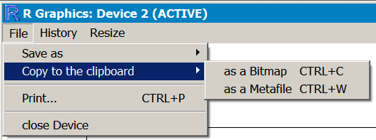
You can simply select the graphics window in R and copy to the clipboard. The clipboard can be pasted into most programs and be recognized as a graphic.

  • On a Mac the graphic will be copied as a PDF object.
  • On Windows you can choose to copy the graphic as a bitmap (Ctrl+C, the default) or as a metafile (Ctrl+W).

In any event the graphic is transferred to your current application as a graphic. The quality of image will depend somewhat on your computer settings but is generally suitable for most daily purposes.

Save graphics from the GUI

You can also save a graphic directly from R using the GUI (assuming you are using Windows or Mac). A browser window opens, allowing you to send the file to a location of your choosing.

  • On a Mac the file will be saved as a PDF.
  • On Windows you can select a file type, there are several options.

The quality of your image (the image size) will depend upon your system settings but you’ll only achieve 72 dpi as a resolution. If you need high-quality images, then you need to use the device drivers.

Device Drivers

The device drivers enable you to send graphics commands directly to a file, rather than the screen. In this way you are able to produce graphics in various formats, with much higher resolution. You can use the device drivers in two main ways:

  • To write an existing graphics window to a file.
  • To write graphics commands direct to a file.

The most commonly used device drivers correspond to popular graphics formats, here are the essentials:

bmp(width = 480, height = 480, units = "px", bg = "white", res)
jpeg(width = 480, height = 480, units = "px", quality = 75, bg = "white", res)
png(width = 480, height = 480, units = "px", bg = "white", res)
tiff(width = 480, height = 480, units = "px", compression, bg = "white", res)

You specify the size of the graphic as width and height. The default is to treat these measurements as pixels, but you can specify units as pixels, inches, centimetres or millimetres. The resolution can be specified, so setting res = 300 will give 300 dpi.

For jpeg you can specify the quality, this sets the approximate percentage filesize so 25 is a smaller file with more compression than 75.

For tiff you can specify a compression, the options are, “none”, “rle”, “lzw”, “jpeg” or “zip”.

You can also make pdf using the pdf() device driver:

pdf(height = 7, width = 7, onefile, paper, colormodel)

For pdf you specify the size in inches. The onefile parameter allows multiple plots to be sent to one file (as separate pages). You can also specify the target page size. The colormodel parameter allows you to specify the colour encoding, the default is “srgb” but you can specify “gray” or “cmyk”.

Copy a graphics device to disk

If you have produced a graphic, in a regular graphic window, and want to save it as a high quality file you can use one of two commands:

dev.copy()
dev.print()

You specify a filename and the type of device you want to make, for example:

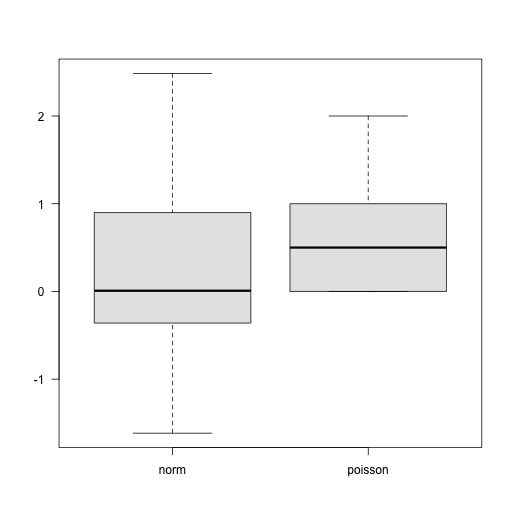
> set.seed(22) # set random number seed
> ## Now make a plot
> boxplot(rnorm(20), rpois(20, 1),
          names  = c("norm", "poisson"),
          las = 1, col = "gray90")

> ## Send to file as PNG
> dev.print(device = png, file = "Myplot.png",
            height = 512, width = 512)
quartz
2

If you use dev.print() the file is written and immediately “closed”. If you use dev.copy() the file it written but not “closed”, which allows you to send additional commands to the file, which must be “closed” using the dev.off() command.

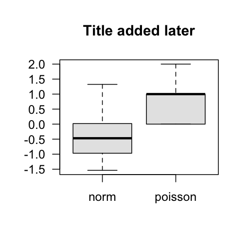
> set.seed(11) # Set random number seed
> ## Make a plot
> boxplot(rnorm(20), rpois(20, 1),
          names  = c("norm", "poisson"),
          las = 1, col = "gray90")

> ## Copy to a file as PNG
> dev.copy(device = png, file = "Myplot.png",
           height = 512, width = 512, res = 150)

quartz_off_screen
3

> ## Add more graphics commands, which go to file not on-screen graphic
> title(“Title added later”)
> ## Close graphic file and finish
> dev.off()

quartz
2

Note that in the preceding example the resolution was set to 150, which affected the size of the text relative to the graphic elements. If you wanted to keep the same relative size as before, set height and width to 512*150/72.

Note that PNG files generally have the background set to “transparent”. If you want to have a plain white background you will need to specify this explicitly in the original graphical command(s) before you use dev.print() or dev.copy(). The simplest way is to set the default:

par(bg = "white")

Now any PNG files you produce will have a white background. Reset to transparent in the same manner.

Send graphics commands direct to a file

If you want to send graphics direct to disk as files you simply issue the appropriate device instruction, which you follow with the graphics commands. Close out the file with dev.off().

> jpeg(file = "MyJpeg.jpg") # Prepare a jpeg file using the defaults
> set.seed(33) # Set random number seed
> ## Make a boxplot, the graphics go direct to file
> boxplot(rnorm(20), rpois(20,1),
          names = c("norm", "poisson"),
          las = 1, col = “cornsilk”)
> dev.off() # Finish and close the file

quartz
2

PDFs are handled generally in the same manner but the parameters are slightly different. Resolution is not an issue so you specify the height and width in inches.

By default, multiple plots are sent to a single file, as separate pages. The default page size (“special”) is set to the same as the graphic size (height and width both 7″ default) but you can specify alternatives, paper = :

  • “a4” or “A4”
  • “letter”
  • “legal” or “us”
  • “executive”

Landscape orientation can be achieved”

  • “A4r”
  • “USr”

These can all be capitalised.

It is possible to change the font(s) used in the file by setting the family parameter. By default, fonts are not embedded so it is best to stick to basic ones e.g.

  • “Helvetica” – the default
  • “AvantGarde”
  • “Bookman”
  • “Courier”
  • “Helvetica-Narrow”
  • “NewCenturySchoolbook”
  • “Palatino”
  • “Times”
## Set PDF to single file using Bookman font family
> pdf(file = "MyPDF.pdf", family = "Bookman)

## Make a couple of plots
> boxplot(rnorm(20), rpois(20,1),
          names = c("norm", "poisson"),
          las = 1, col = "cornsilk")
> boxplot(rnorm(20), rpois(20, 1),
          names  = c("norm", "poisson"),
          las = 1, col = "gray90")

## Close the file and finish
> dev.off()

pdf
3

The preceding example should produce two boxplots in a single file. The size of the paper will be the default (7”). The Bookman font family was used.

Multiple plot files

If you want to produce multiple plots it is not necessary to issue a separate filename for each plot. You can simply add an index to the filename; something like %03d will produce three-digit integer values in the filename:

## Start a jpeg device with default size but an indexed name
> jpeg(file = "MyJpeg%03d.jpg")

## Make a plot
> boxplot(rnorm(20), rpois(20, 1),
          names  = c("norm", "poisson"),
          las = 1, col = "gray90")
## Add a title
> title(main = "Fig. 1")

## Start a new plot, this closes the previous
> boxplot(rnorm(20), rpois(20,1),
          names = c("norm", "poisson"),
          las = 1, col = "cornsilk")
> title(main = "Fig. 2")

## Close the last device and finish the file
> dev.off()

null device
1

The preceding example should produce two plots, one called MyJpeg001.jpg and another MyJpeg002.jpg. Note that the first file is “closed” when you issue a graphical command that would create a new plot. So if you want to add titles or similar, then you should do it before starting the next graphic, you cannot go back.

Writing scripts

A script is simply a text file containing a series of R commands. You store the file and run it using the source() command. You have two main choices for writing of script files: use the built-in script editor or an outside editor. The GUI for Windows and Mac incorporates a script editor but only the Mac supports syntax highlighting.

To start a new script:

  • Win: File >New script
  • Mac: File >New Document

You can open a script in any text editor of course. In Windows the Notepad++ program is a simple editor with syntax highlighting. On the Mac the BBEdit program is highly recommended. On Linux there are many options, the default text editor will often support syntax highlighting, Geany is one IDE that not only has syntax highlighting but integrates with the terminal.

The RStudio IDE is very capable and makes a good platform for using R for any OS. The script editor has syntax highlighting.

If you start to get serious about R coding, then the Sublime Text editor is worth a look. This has versions for all OS and syntax highlighting for R and many other languages.

Working Directory

R uses a working directory, where it stores files and where it looks for items to read. You can see the current working directory using getwd():

> getwd()
[1] "/Users/markgardener"

> getwd()
[1] "C:/Users/Mark/Documents"

So, whenever you specify a filename it will be output to the working directory unless you specify a “complete” location, that is the full directory path. There is more about the working directory in the page about Reading.

The 3 Rs Reading

You can probably think of “reading matter” as being one of three sorts:

  • data
  • R objects
  • scripts

Data is a general term and by this I mean numbers and characters that you might reasonably suppose could be handled by a spreadsheet. Your data are what you use in your analyses.

R objects may be data or other things, such as custom R commands. They are usually stored (on disk) in a format that can only be read by R but sometimes they may be in text form.

Scripts are collections of R commands that are designed to be run “automatically”. They are generally saved (on disk) in text format.

Reading – using the keyboard

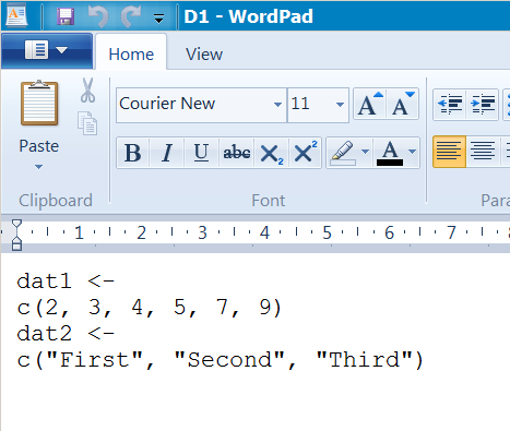
The simplest way to “read” data into R is to type it yourself using the keyboard. The c() command is the simplest method. Think of c for “combine” or “concatenate”. To make some data you type them in the command and separate the elements with commas:

> dat1 <- c(2, 3,4,5, 7, 9)
> dat1
[1] 2 3 4 5 7 9

Note that R ignores any spaces.

If you want text values you will have to enclose each element in quotes, you can use single or double quotes as long as they “match”.

> dat2 <- c("First", 'Second', "Third")
> dat2
[1] "First"  "Second" "Third"

When you “display” your text (character) data R includes the quotes (R always shows double quotes). You can use the c() command to join many items, not just numbers or character data. However, here you’ll see it used simply for “reading” regular data. The result of the c() command is generally a vector, a 1-dimensional data object. You can add to existing data but if you “mix” data types you may not get what you expect:

> dat3 <- c(1, 2, 3, "First", "Second", "Third")
> dat3
[1] "1"      "2"      "3"      "First"  "Second" "Third"

R has converted the numbers to text (character) values.

Use scan()

Typing the commas and/or quotes can be a pain, especially when you have more than a few items to enter. This is where the scan() command comes in useful. The scan() command is quite flexible and can read the keyboard, clipboard and files on disk. The simplest way to use scan() is for entering numbers. You invoke the command and then type numerical values, separated by spaces. You can press the ENTER key at any time but the data entry will not stop until you press ENTER on a blank line (i.e. you press ENTER twice).

> dat4 <- scan()
1: 3 6 7 12 13 9 8 4
9: 7 7 8 12 5
14: 4
15:
Read 14 items
> dat4
[1]  3  6  7 12 13  9  8  4  7  7  8 12  5  4

In the preceding example eight values were typed and then the ENTER pressed. You can see that the R cursor changes from the >. This helps you to keep track of how many items you’ve typed. After the first eight items we typed five more (the line beginning with 9:) and then pressed ENTER again. R displayed 14: to show us that the next item would be the 14th. One value was typed and then ENTER pressed twice to complete the process.

If you want to type character data you must add the what = “character” parameter to the command, then R “knows” what to expect and you do not need to type quotes:

> dat5 <- scan(what = "character")
1: Mon Tue Wed Thu Fri
6: Sat Sun
8:
Read 7 items
> dat5
[1] "Mon" "Tue" "Wed" "Thu" "Fri" "Sat" "Sun"

You can specify the separator character using the sep = parameter, although the default space seems adequate! If you are so inclined, you can also specify an alternative character for the decimal point via the dec = parameter.

> dat6 <- scan(sep = "", dec = ",")
1: 34 4,6
3: 1,4 7,34
5:
Read 4 items 

> dat6
[1] 34.00  4.60  1.40  7.34

Notice that the default is actually two quotes with no space between! The sep and dec parameters are more useful for reading data from clipboard or disk files, as you will see next.

Reading – using the clipboard

The scan() command can read the clipboard. This can be useful to shift larger quantities of data into R. You’ll probably have data in a spreadsheet but any program that can display text will allow you to copy to the clipboard.

Data in a spreadsheet

If you open the data is a spreadsheet then you can copy a column of data and use scan() as if you were going to type it from the keyboard. You do not need to specify the separator character (the default “” will suffice) when using a spreadsheet but you can specify the decimal point character if necessary.

Opening a text file in Excel allows you to see the data separator.

If you need to copy items by row, then you cannot do it using a spreadsheet unless you have a Mac. To get a column of data into R you simply copy the data to the clipboard:

If you need to copy items by row, then you cannot do it using a spreadsheet unless you have a Mac. To get a column of data into R you simply copy the data to the clipboard:

Then switch to R and use the scan() command:

> dat7 <- scan()
1: 34
2: 32
3: 30
4: 36
5: 36
6: 36
7: 41
8: 35
9: 30
10: 34
11:
Read 10 items

To finish you press ENTER on a blank line, this means you could copy more data and append it if you wish.

Multiple paste

Once you’ve pasted some data into R using scan() you finish the operation by pressing ENTER on a blank line. Usually this means that you have to press ENTER twice. If you want to add more data, you can simply press ENTER once and copy/paste more stuff.

Rows of data

If the data are in a spreadsheet or are separated by TAB characters you cannot read rows of data (unless you have a Mac). If you open the data in a text editor (Notepad or Wordpad for example) then you’ll be able to select and copy multiple rows of data as long as the items are not TAB separated. In the following example Notepad is used to open a comma separated file. Several rows are copied to the clipboard:

The scan() command can now be used, using the sep = “,” parameter as the data are comma separated:

> dat8 <- scan(sep = “,”)
1: 34,35,33,26,35,35,35,32,38,29
11: 32,34,33,29,37,37,31,37,31,28
21: 30,38,34,33,33,32,29,35,29,30
31:
Read 30 items

In total 30 data elements were read (note that the data are read row by row). ENTER was pressed after the first paste operation but you could add more data, completing data entry by pressing ENTER on a blank line.

End of Line characters

Text files can be split into lines using several methods. In general Linux and Mac use LF whereas Windows uses CR/LF (older Mac used CR). This can mean that if you use Windows and Notepad to open a file the data are not displayed “neatly” and everything appears on one line.

Wordpad is built in to Windows and this will handle alternative line endings quite adequately.


The Notepad++ program will also handle alternative end of line characters and allows you to alter the EOL setting for a file. It also supports syntax highlighting.

On a Mac the default TextEdit app will deal with alternative line endings but BBEdit is a useful editor, which also supports syntax highlighting.

If you use Linux, then it is likely that your default text editor will deal with any EOL setting and also allow you to alter the encoding.

Converting separators

If you have data in TAB separated format and want to convert it to simple space separated or comma separated format, then the easiest way is to open the data in your spreadsheet. Then use File > Save As.. to save the file in a new format.

The preceding example shows Excel 2010 but other versions of Excel have similar options. OpenOffice and LibreOffice also allow saving of files in various formats.

The TAB separated format is useful for displaying items for people to read but not so good for copy/paste. Comma separated files are generally most useful and can be produced by many programs. Space separated files are somewhere in-between.

Of course there is no need to convert TAB separated files, they are only a problem if you are going to use copy/paste. R can handle TAB separators quite easily if the file is to be read directly from disk.

Reading – from disk files

If you have a data file on disk, you can read it into R without opening it first. There are two main options:

  • the scan() command
  • the table() command

Generally speaking you’d use scan() to read a data file and make a vector object in R. That is, you use it to get/make a single sample (a 1-D object). You use the read.table() command to access a file with multiple columns, each one representing a separate sample or variable. The result is a data.frame object in R (a 2-D object with rows and columns).

The read.table() command has many options and there are several convenience functions, such as read.csv(), allowing you to read some popular formats with appropriate defaults.

Use scan() to read a disk file

To get scan() to read a file from disk you simply specify the filename (in quotes) in the command. You can set the separator character and decimal point character as appropriate using sep = and dec = parameters. If you are using Windows or Mac you can use file.choose() instead of the filename:

> dat8 <- scan(file.choose())
Read 100 items

The file.choose() part opens a browser-like window and permits you to select the file you require.

The file selected in the preceding example was called L1.txt and you can view this in your browser. It is simply separated with spaces. The result is a vector of 100 data items even though the original file seems composed of ten columns.

If you have a file separated with commas, like L2.txt, then you simply specify sep = “,” like so:

> dat9 <- scan(file.choose(), sep = “,”)
Read 100 items

The result is the same, a vector of 100 items. When the separator character is a TAB (e.g. L3.txt) you can use the sep = “\t” parameter.

> dat10 <- scan(file.choose(), sep = “\t”)
Read 100 items

Sometimes your data may include comments, these are helpful to remind you what the data were but you need to be able to deal with them.

Comments in data files

It is helpful to include comments in plain data files. This helps you (and others) to determine what the data represent without having to look elsewhere. The scan() command can “read and ignore” rows that are “flagged” as comments.

You can set rows that begin with a special character to be ignored using the comment.char = parameter. Of course you could use any character as a comment marker but in R the # is used so that would seem sensible.

> dat11 <- scan(file.choose(), comment.char = “#”)
Read 100 items

Have a look at the L1c.txt file. This has three comment lines at the start. The file itself is space separated.

Working directory

If you do not use file.choose() or you have Linux OS then you’ll have to specify the filename exactly (in quotes). R uses a working directory, where it stores files and where it looks for items to read. You can see the current working directory using getwd():

> getwd()
[1] "/Users/markgardener"

> getwd()
[1] "C:/Users/Mark/Documents"

You can set the working directory to a new folder by specifying the new filepath (in quotes) in the setwd() command:

> getwd() # Get the current wd
[1] "/Users/markgardener"

> setwd("Desktop") # Set to new value

> getwd() # Check that wd is set as expected
[1] "/Users/markgardener/Desktop"

> setwd("/Users/markgardener") # set back to original

> getwd()
[1] "/Users/markgardener"

You can “reset” your working directory using the tilde:

> setwd("~")
> getwd()
[1] "/Users/markgardener"


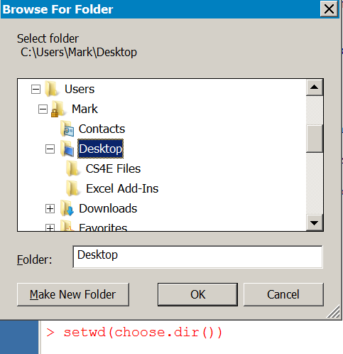
If you use Windows you can use choose.dir() in the setwd() command to interactively set a working directory like so:

> setwd(choose.dir())

Reading from URL

You can use scan() to read a file directly from the Internet if you have the URL, use that instead of the filename. The URL needs to be complete and in quotes:

Note that you cannot use spaces in the URL. If you copy/paste the URL from the website any spaces will be shown as %20:

> dat12 <- scan(file = “http://www.mysite/data%20files/test.txt”)
Read 100 items

You can use all the other parameters that you’ve seen before. Have a go yourself using these files:

  • txt – a space separated file
  • txt – a space separated file with comments
  • txt – a comma separated file
  • txt – a TAB separated file

If you right-click a hyperlink you can copy the URL to the clipboard.

Reading multi-column files

The scan() command reads files and stores the result as a vector. However, many data files will contain multiple columns that represent different variables. In this case you don’t want a single vector item but a data.frame, which reflects the rows and columns of the original data.

The read.table() command is a general tool for reading files from disk (or URL) and making data.frame results. You can set decimal point characters and separators in a similar way to scan(). However, you can also set names for columns and/or rows if required.

There are several convenience commands to help in reading “popular” formats:

  • csv() – this reads comma separated files
  • csv2() – uses semi-colon as the separator and the comma as a decimal point
  • delim() – uses TAB as a separator
  • delim2() – uses TAB as a separator and comma as decimal point

The read.csv() command is probably the most generally useful command as CSV format is the most widely used and can be saved by most programs.

The files L1.txtL2.txtL3.txt and L1c.txt are all ten columns (and 10 rows) in size. Previously you saw how the scan() command can read these files and create a single sample, as a vector object, from the data. By contrast, the read.table() command treats each column as a separate variable:

> dat12 <- read.table(file = “L1.txt”)
> dat12
   V1 V2 V3 V4 V5 V6 V7 V8 V9 V10
1  34 35 33 26 35 35 35 32 38  29
2  32 34 33 29 37 37 31 37 31  28
3  30 38 34 33 33 32 29 35 29  30
4  36 32 31 33 35 35 31 34 29  29
5  36 34 37 28 27 32 28 32 36  32
6  36 31 33 38 33 32 36 33 34  31
7  41 34 30 27 34 34 29 27 37  31
8  35 34 27 35 28 31 31 36 32  32
9  30 33 36 34 29 33 28 34 37  34
10 34 33 31 30 36 26 29 35 34  35

In the preceding example the L1.txt file was used, this is space separated so the default sep = ” ” need not be specified. Notice how R has “invented” names for the columns (the original file does not have column names). If the data are comma separated you can use the sep = “,” parameter:

> dat13 <- read.table(file = "L2.txt", sep = ",")

Any comment lines are dealt with by the comment.char parameter:

> dat14 <- read.table(file = "L1c.txt", sep = "", comment.char = "#")

The read.table() command assumes that there are no column names in the original data. You can assign names as part of the read.table() command using the col.names parameter. You need to specify exactly the correct number of names.

> cn = paste("X", 1:10, sep = "") # Make some names
> cn
[1] "X1"  "X2"  "X3"  "X4"  "X5"  "X6"  "X7"  "X8"  "X9"  "X10"

> dat15 <- read.table(file = "L1.txt", col.names = cn)

> head(dat15, n = 3)
   X1 X2 X3 X4 X5 X6 X7 X8 X9 X10
1  34 35 33 26 35 35 35 32 38  29
2  32 34 33 29 37 37 31 37 31  28
3  30 38 34 33 33 32 29 35 29  30

You can always alter the names afterwards if you prefer.

Column headings

In most cases your data will contain column headings. You can set these column headers using header = TRUE in the read.table() command.

> dat16 <- read.table(file = “L6.txt”, header = TRUE)
> dat16
   Smpl1 Smpl2 Smpl3 Smpl4 Smpl5 Smpl6 Smpl7 Smpl8 Smpl9 Smpl10
1     34    35    33    26    35    35    35    32    38     29
2     32    34    33    29    37    37    31    37    31     28
3     30    38    34    33    33    32    29    35    29     30
4     36    32    31    33    35    35    31    34    29     29
5     36    34    37    28    27    32    28    32    36     32
6     36    31    33    38    33    32    36    33    34     31
7     41    34    30    27    34    34    29    27    37     31
8     35    34    27    35    28    31    31    36    32     32
9     30    33    36    34    29    33    28    34    37     34
10    34    33    31    30    36    26    29    35    34     35

The file L6.txt is space separated. If you have TAB or comma separated you simply alter the sep parameter as appropriate. Try the following files for yourself:

  • txt – a comma separated file
  • txt – a TAB separated file
  • txt – a space separated file

Use “\t” to represent a TAB character:

> dat17 <- read.table(file = "L5.txt", header = TRUE, sep = "\t")

Note that R will check to see that the column names are “valid”, and will alter the names as necessary. You can over-ride this process using the check.names = FALSE parameter. This can be useful to allow numbers to be used as headings (such as years, e.g. 2001, 2002). However, it is a good idea to check the original datafile first.

Sometimes your data will have row headings, if so you will need an additional parameter, row.names.

Row headings

If your data contains row headings you can use the row.names parameter to instruct the read.table() command which column contains the headings (usually the first).

> dat18 <- read.table(file = “L7.txt”, sep = “”, header = TRUE, row.names = 1)
> dat18
      Smpl1 Smpl2 Smpl3 Smpl4 Smpl5 Smpl6 Smpl7 Smpl8 Smpl9 Smpl10
Obs1     34    35    33    26    35    35    35    32    38     29
Obs2     32    34    33    29    37    37    31    37    31     28
Obs3     30    38    34    33    33    32    29    35    29     30
Obs4     36    32    31    33    35    35    31    34    29     29
Obs5     36    34    37    28    27    32    28    32    36     32
Obs6     36    31    33    38    33    32    36    33    34     31
Obs7     41    34    30    27    34    34    29    27    37     31
Obs8     35    34    27    35    28    31    31    36    32     32
Obs9     30    33    36    34    29    33    28    34    37     34
Obs10    34    33    31    30    36    26    29    35    34     35

Notice that the default is sep = “”, this is used for space separated files but you do not need to put a space between the quotes! The row.names parameter needs a single numerical value, to identify the column that contains the headings. If the separator character is different you simply change the sep parameter. Try the following files for yourself:

  • txt – a space separated file
  • txt – a comma separated file
  • txt – a TAB separated file

All these files contain both row and column names.

Usually you give a column number in the row.names parameter. However, there are several ways to specify the row headings:

  • A number corresponding to the column containing the names
  • The name of the column header (in quotes) containing the names
  • A vector of names to use as row headings/names

If the data are simple space delimited and contain column headings in all columns except the first (so column 1 is 1 element shorter than the other columns) it will be treated as a column of row headings (that is you do not need to specify row.names). In practice it is best to use a definite value for row.names. You can “force” simple numbered rows by setting row.names = NULL.

The read.xxx() convenience commands

There are four convenience functions, designed to make things a bit easier when dealing with some common formats.

  • csv() – this reads comma separated files
  • csv2() – uses semi-colon as the separator and the comma as a decimal point
  • delim() – uses TAB as a separator
  • delim2() – uses TAB as a separator and comma as decimal point

All these commands have header = TRUE and comment = “”, set as default. This makes things simpler, the following commands achieve the same result:

> read.csv("L8.txt", row.names = 1)
> read.table("L8.txt", sep = ",", header = TRUE, row.names = 1)
> read.delim2("L8.txt", sep = ",", header = TRUE, row.names = 1, dec = ".")

You use any of the read.xxxx() commands as long as you over-ride the defaults. See the help entry for read.table() by typing help(read.table) in R.

Column formats

When you read a multi-column file into R the various columns are “inspected” and converted to an appropriate type. Generally, any character columns are converted to factor variables whilst numbers are kept as numbers. This is usually an acceptable process, since in most analytical situations you want character values to be treated as variable factors.

However, there may be times when you want to alter the default behaviour and read columns in a particular format. Here is a data file with several columns:

     count treat day int
obs1    23    hi mon   1
obs2    17    hi tue   1
obs3    16    hi wed   1
obs4    14    lo mon   2
obs5    11    lo tue   2
obs6    19    lo wed   2

The first column can act as row headers/names. The “count” column is fairly obviously a numeric value. The “treat” column is an experimental factor whilst “day” is simply a label (text). The “int” column is intended to be a treatment label. It is common in some branches of science to use plain numerical values as treatment labels.

When you read this file into R the columns are “interpreted” like so:

> df1 <- read.csv(“L11.txt”, row.names = 1)
> df1
     count treat day int
obs1    23    hi mon   1
obs2    17    hi tue   1
obs3    16    hi wed   1
obs4    14    lo mon   2
obs5    11    lo tue   2
obs6    19    lo wed   2
> str(df1) # Examine object structure
‘data.frame’:     6 obs. of  4 variables:
$ count: int  23 17 16 14 11 19
$ treat: Factor w/ 2 levels "hi","lo": 1 1 1 2 2 2
$ day  : Factor w/ 3 levels "mon","tue","wed": 1 2 3 1 2 3
$ int  : int  1 1 1 2 2 2

The file L11.txt now appears to have the column “day” converted to a factor variable and the “int” column is a number rather than a factor.

You can control the interpretation in several ways using parameters in the read.xxxx() commands:

  • stringsAsFactors – set this to FALSE to keep character columns as character variables
  • is – give the column numbers to keep “as is” and not convert
  • colClasses – give a vector of character strings corresponding to the classes required

The stringsAsFactors parameter is the most “simple” and is over-ridden if one of the others is used. It provides “blanket coverage” and operates on the entire data file being read:

> df2 <- read.csv("L11.txt", row.names = 1, stringsAsFactors = FALSE)
> str(df2)
‘data.frame’:     6 obs. of  4 variables:
$ count: int  23 17 16 14 11 19
$ treat: chr  "hi" "hi" "hi" "lo" ...
$ day  : chr  "mon" "tue" "wed" "mon" ...
$ int  : int  1 1 1 2 2 2

The as.is parameter operates only on the columns you specify – don’t forget that the column containing row names is column 1:

> df3 <- read.csv("L11.txt", row.names = 1, as.is = 4)

> str(df3)
‘data.frame’:     6 obs. of  4 variables:
$ count: int  23 17 16 14 11 19
$ treat: Factor w/ 2 levels "hi","lo": 1 1 1 2 2 2
$ day  : chr  "mon" "tue" "wed" "mon" ...
$ int  : int  1 1 1 2 2 2

All other parameters work as they did before so if you have a space or TAB separated file for example you can use the sep parameter as necessary. Try these files if you want some practice:

  • txt – a TAB separated file with row names
  • txt – a comma separated file with row names
  • txt – a space separated file with row names

Using the colClasses parameter gives you the finest control over the columns. You must specify (as a character vector) the required class for each column. In the example here you would want “count” to be an integer (or simply numeric), “treat” to be a factor, “day” to be character and “int” to be a factor (remember we said this represented an experimental treatment). Don’t forget the column of row names – use character for these:

## Define the column classes
> cc <- c("character", "integer", "factor", "character", "factor")

## Read the file and set column classes
> df4 <- read.csv("L11.txt", row.names = 1, colClasses = cc)

> str(df4)
‘data.frame’:     6 obs. of  4 variables:
$ count: int  23 17 16 14 11 19
$ treat: Factor w/ 2 levels "hi","lo": 1 1 1 2 2 2
$ day  : chr  "mon" "tue" "wed" "mon" ...
$ int  : Factor w/ 2 levels "1","2": 1 1 1 2 2 2

You can of course set the columns of the resulting data.frame afterwards but it makes sense to do this right at the start.

Reading R objects from disk

R objects can be stored on disk in one of two formats:

  • Binary – usually .RData files that are encoded and only readable by R
  • Text – plain text files that can be read by text editors (and R)

Generally speaking an R object is something you see when you use the ls() command, the objects() command does the same thing and the two are synonymous. Any R object can be saved to disk.

Usually text files will be “raw data” files and scripts (collections of R commands that are executed when the script is run). However, it is possible to have text versions of other R objects.

Binary files are generally used to keep custom commands, data and results objects. Often you’ll have several objects bundled together.

There are several ways to get these objects into R.

Use the OS to open R objects

In Windows and Mac you can usually open .RData and .R files directly from the operating system. Usually .RData files are associated with R so if you double click a file it will open R and load the objects it contains. There are two scenarios:

  • R is already running
  • R is not running

You get a different result in each case.

If R is not running

If R is not running and you double click a .RData file, R will open and read the objects contained in the file. In addition, the working directory will be set to the folder containing the .RData file.

So, if you double click the file or drag its icon to the R program icon (shortcut on desktop, taskbar or dock) then R will open. You can check the working directory, which should point to the folder containing the file you opened:

> getwd()
[1] "Y:/Dropbox/Source data files/R Source files"

In Windows if you drag the icon to the R program icon you can “pin” it to the taksbar, this can allow you to open a data file later with a right click of the taskbar icon:

Files that are stored in text format, usually with the .R extension, are handled differently. Since they are plain text the default program may well be a text editor, depending what is installed on your computer. You can right click a file or (in Windows) click the Open button on the menu bar to see what programs are available.

In Windows you will probably have to open the file with a text editor of some kind. If you have the RStudio IDE you can select to open the file in this, RStudio will run and your file will appear in the script window. Note that if R has saved a text representation of objects the file will have Unix-style EOL characters (LF), and Notepad will not display the data properly. Wordpad or Notepad++ are fine though.

In Mac you may have the file associated with a text editor or with R. If you open the file using R then the text appears in the script editor window.

If you use Linux you cannot open .RData files from the OS. R text files can be opened in a text editor. If you use RStudio IDE then .RData or .R files can be opened (in RStudio) from the OS.

So, .RData objects can be read into R directly via the OS but text representations of R objects (.R files) cannot.

If R is already running

If R is already running when you try to open an .RData file by double clicking, what happens depends on the OS.

  • In Windows R opens in a new window
  • In Mac R appends the data to the current workspace

In Windows you get another R window, the data in the .RData file is loaded and the working directory set to the folder containing the file, just as if R had not been open.

In Mac the data are appended to the current workspace and the working directory remains unchanged.

If you are using Windows and want to append the data to your current workspace then you must drag the file icon to the running R program window and drop it in. If you drag to the taskbar and wait a second, the program window will open and you can drop the file into the console.

Something similar happens on a Mac, you can drag a file to the dock icon or into the running R console window.

Get binary files with load() command

You can load .RData files directly from within R using the load() command. You need to supply the name of the file (in quotes) although in Windows or Mac you can use file.choose() instead. Any filenames must include the full file path if the file is not in your working directory.

> ls()
character(0)

> load(file = "Obj1.RData")
> ls()
[1] "data_item_1" "data_item_2"

In Windows and Mac you can also use a menu:

  • Mac: Workspace > Load Workspace File…
  • Win: File > Load Workspace…

The data are appended to anything in the current workspace and any items that are named the same as incoming items are overwritten without warning. The working directory is unaffected.

If you want a practice file, try the Obj1.RData file. You’ll have to download it, although you could try loading the file using the URL.

Get text files with dget() or source() command

R can make text representations of objects. Generally, there are two forms:

  • Un-named objects
  • Named objects

You’ll need to use the dget() or source() commands to read these text files into R.

Un-named R objects as text

Un-named objects are created using the dput() command and are text representations of single objects. The text can look slightly odd, see the D2.R example:

structure(c(1L, 1L, 1L, 2L, 2L, 2L), .Label = c("high", "low" ), class = "factor")

To read one of these objects into R you need the dget() command. Since the object is un-named in the text file you’ll need to assign a name in the workspace:

> ls() # Check what is in workspace
character(0)

> fac1 = dget(file = "D2.R") # Get object

> fac1
[1] high high high low  low  low
Levels: high low

Note that there is no GUI menu command that will read this kind of text object, you have to use dget(). Other text representations look more like regular R commands (i.e. the objects are named), you need a different approach for these.

Named R objects as text

Some R text objects look more like regular R commands. These can be saved to disk using the dump() command, which can save more than one object at a time (unlike the dput() command). An example is the D1.R file:

dat1 <- c(2, 3, 4, 5, 7, 9)
dat2 <- c("First", "Second", "Third")

The D1.R file was created using the dump() command to save two objects (dat1 and dat2).

To get these into R you need the source() command:

> ls() # Check what is in workspace
character(0)

> source(file = "D1.R") # Get the objects

> ls()
[1] "dat1" "dat2"

> dat1 ; dat2
[1] 2 3 4 5 7 9
[1] "First"  "Second" "Third"

In the preceding example the file was named explicitly but in Windows or Mac you can use file.choose() instead (also in Linux if you are running the RStudio IDE). Notice that you do not need to name the objects, the data file already has assigned names.

It is possible to use menu commands in Windows or Mac to get this kind of file into R:

  • Win: File > Source R code…
  • Mac: File > Source File…

This kind of text file is more like a series of R commands, which would generally be called an R script. Such script files are very useful, as you can use them for many purposes, such as making a custom calculation that can be run whenever you want.

R script files

R script files are simply a series of R commands saved in a plain text file. When you use the source() command, the commands are executed as if you had typed them into the R console directly.

Generally speaking you’ll want to “look over” the script before you it. This usually means opening the file in a text editor. Some text editors “know” the R syntax and can highlight the text accordingly, making the script easier to follow. Both Windows and Mac R GUI have a script editor but only the Mac version has syntax highlighting.

To open a script file in the R GUI use the File menu:

  • Win: File > Open script…
  • Mac: File > Open Document…

You can open a script in any text editor of course. In Windows the Notepad++ program is a simple editor with syntax highlighting. On the Mac the BBEdit program is highly recommended. On Linux there are many options, the default text editor will often support syntax highlighting, Geany is one IDE that not only has syntax highlighting but integrates with the terminal.

The RStudio IDE is very capable and makes a good platform for using R for any OS. The script editor has syntax highlighting.

If you start to get serious about R coding, then the Sublime Text editor is worth a look. This has versions for all OS and syntax highlighting for R and many other languages.

Reading other types of file

R cannot read other file types “out of the box” but there are command packages that will read other files. Two commonly used ones are foreign and xlsx.

Package foreign

The foreign package can read files created by several programs including (but not limited to):

  • SPSS – files made by save or export can be read
  • dBase – .dbf files, which are also used by other programs in the XBase family
  • MiniTab – .mtp MiniTab portable worksheets
  • Stata – .dta files up to version 12
  • Systat – .sys or .syd files
  • SAS – XPORT format files (there is also a command to convert SAS files to XPORT format)

There are various limitations, the package has not been updated for a while. In general, it is best to save data in CSV format, which most programs can do. If you get sent a file in an odd format, then you can ask the sender to convert it or try the package and see what you can do. The index file of the package help should give you a fair indication of what is available.

Package xlsx

The xlsx package reads Excel files. The main command is read.xlsx(), which has various options for Excel formatted files. There is also a read.xlsx2() command, this is more or less the same but uses Java more heavily and is probably better for large spreadsheets.

The essentials of the command are:

read.xlsx(file, sheetIndex, sheetName = NULL)

You provide the filename (file) and either a number corresponding to a worksheet (sheetIndex) or the name of the worksheet (sheetName = “worksheet_name”). You can use file.choose() to select the file interactively (except on Linux).

There is also a parameter colClasses, which you can use to force various columns into the class you require. You give a character vector containing the classes you want – they are recycled as necessary. In general, you should try a regular read and see what classes result. If there are some “oddities” you can either alter them in the imported object or re-import and set the classes explicitly.