The usual way of creating a chart in Excel is to highlight your data then click the appropriate chart button from the Insert menu. However, the resulting graph often appears in a layout that is not what you wanted and you have to spend time editing the graph. A cleaner approach is to create an empty graph and add the data to it and build the graph you want from scratch. This is more like the “old” way of doing things when you had the “chart wizard”.

1. Click once in your spreadsheet to “set” the current cell. Make sure you click away from any data as Excel will “search” around the current cell and automatically select anything it finds.
2. Click on the Insert tab to bring up the graph options.
3. Click the button appropriate to the chart you want.
4. A blank chart now appears; use the Select Data button to begin the process of building your chart.

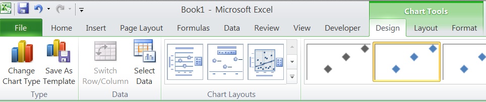
If you don’t see the button, then make sure you click once on the blank chart then select the Home > Chart Tools > Design menu. You are now able to select the data you want and can ensure that the x and y axes are the right way around for example. More on building charts in the future. See our Tips & Tricks pages for more.