Welch two-sample t-test
Exercise 7.1.1
Statistics for Ecologists (Edition 2) Exercise 7.1.1
This exercise is concerned with using Excel for the t-test in Chapter 7 (Section 7.1). In particular you’ll see how to modify the degrees of freedom for cases when the variance of two samples is not equal (which is often).
Welch two-sample t-test
Introduction
The t-test is used to compare the means of two samples that have a normal (parametric or Gaussian) distribution. The “classic” t-test has two major variants:
- Assumption of equal variance for the two samples.
- Adjustment of degrees of freedom (Satterthwaite modification).
In the first case the common variance is calculated and used in place of the variance in the regular formula. The calculation for this is relatively simple but it is also pointless, since you still have to determine the variance of the two samples.
The most commonly used modification is to adjust the degrees of freedom to make the result of the t-test a little more conservative. The degrees of freedom are reduced slightly using the Satterthwaite modification. This version of the t-test is generally called the Welch 2-sample t-test.
The calculations are relatively easy. You can then use the modified df for looking up critical values or for computing the exact p-value. The Welch 2-sample t-test is carried out by default in R via the t.test() command. In Excel the TTEST function will give you the exact p-value but it will not provide the modified degrees of freedom.
The Excel functions TDIST and TINV will give incorrect results as they assume equal variance and use un-modified degrees of freedom. This exercise works through the t-test and shows how to use the Satterthwaite modification to alter degrees of freedom. This allows you to get the “proper” result in Excel. The calculation matches that used in the Analysis ToolPak, which is available in Windows versions of Excel and later Mac versions.
The exercise uses the data that you can see in the following table:
Abundance of R. repens in ridges and furrows of a mediaeval meadow
| A | B | C | |
| 1 | ridge | furrow | |
| 2 | 4 | 9 | |
| 3 | 3 | 8 | |
| 4 | 5 | 10 | |
| 5 | 6 | 6 | |
| 6 | 8 | 7 | |
| 7 | 6 | ||
| 8 | 5 | ||
| 9 | 7 |
The data show the abundance of a plant species in two different habitats. The two samples are small but are normally distributed. You can get a copy of the data in Excel .xlsx format here: ridge furrow.xlsx.
Calculation
The calculation of the modified degrees of freedom are in two parts. To start with you determine a statistic called u, which you can think of as a kind of proportion (it varies from 0–1).

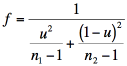
Once you have a value for u, you can determine f, the modified degrees of freedom.

The formula gives the same value whichever sample you choose to be #1 and which #2. The df are reduced slightly from the original: original df = (n1 – 1 + n2 – 1).
Once you have a modified df you can use it to look up the critical value, either in a table or using the TINV function in Excel. The equivalent in R would be the qt() function.
Carry out basic t-test
Start by opening the ridge furrow.xlsx data file. Go to the Data worksheet (the t-test completed worksheet is provided for you to check your results). The two samples are in columns B and C.
- In cell A10 type a label for the number of observations in each sample, “n” will do nicely.
- In cell B10 type a formula to determine the number of observations =COUNT(B2:B9)
- Copy cell B10 into C10 so that you have a result for each sample
- In cell A11 type a label for the mean values, “mean” will do fine.
- In cell B11 type a formula to work out the mean = AVERAGE(B2:B9).
- Copy cell B11 into C11 so that you have a result for each sample.
- In cell A12 type a label for the variance, “variance” seems logical.
- In cell B12 type a formula to calculate the variance =VAR(B2:B9)
- Copy the variance formula from B12 to C12.
- In A13 type a label for the t-value, “t” or “t-value” will do.
- In cell B13 type a formula to work out the value of t: =ABS(B11-C11)/SQRT(B12/B10+C12/C10)
- In A15 (yes, leave a blank row) type a label “p-value”.
- In B15 type a formula to work out the p-value based on the t you calculated: =TDIST(B13,B10+C10-2,2)
- The p-value from step 13 (p = 0.019) is based on equal variance (and un-modified degrees of freedom) and so is not really correct. Carry on and calculate a critical value.
- In A17 type a label “t-crit”.
- In B17 type a formula to work out a critical value for t: =TINV(0.05,B10+C10-2)
The critical value from step 15 (t = 2.201) is also based on equal variance and un-modified degrees of freedom.
- In A18 type another label “p-value”, for the exact p-value computed by Excel’s TTEST function.
- In B18 type a formula to compute the exact p-value for a t-test with un-equal variance: =TTEST(B2:B9,C2:C6,2,3)
Note that the TTEST function gives a more conservative p-value (of 0.023) because it has calculated the modified degrees of freedom. However, you cannot extract the df directly and will have to compute it if you want to report a more appropriate critical value you’ll need to compute it longhand.
Compute modified degrees of freedom
The calculation of the modified degrees of freedom (Satterthwaite modification) will require some simple maths using the equations from earlier:
- In Cell A20 type a label “u” for the result of the first calculation.
- In B20 type a formula to calculate u: =(B12/B10)/((B12/B10)+(C12/C10)).
- In A21 type a label “f” for the result of the second calculation.
- In B21 type a formula to calculate f: =1/(((B20^2)/(B10-1))+(((1-B20)^2)/(C10-1)))
- Your result from step 21 should be 8.733. Excel cannot deal with degrees of freedom that are not integer values so you need to round up (Excel always rounds the df value upwards):
- In A22 type a label “df” for the integer df result.
- In B22 type a formula to round up the value from step 21: =CEILING(B21,1)
- Now you have a modified df (df = 9) you can use it to calculate a critical value. You can also see how the modified df can be used in TINV and TDIST functions.
- In A24 type a label “t-crit” for the new critical value.
- In B24 type a function to compute the critical value based on the new df: =TINV(0.05,B22)
- Note that the critical value from step 25 (t = 2.262) is higher than the value from step 15, and so a bit more conservative.
- In A25 type a label “p-value” for the exact p-value based on the modified df.
- In B25 type a formula to work out the exact p-value: =TDIST(B13,B22,2)
Note that the exact p-value from step 27 (p = 0.022) is very similar to that you obtained from the TTEST function in step 17. If you have a p-value you can get the value of t but only if you have the modified degrees of freedom.
- In A26 type a label “t-value” for the t calculation.
- In B26 type a formula that calculates the value of t based on the p-value and modified df: =TINV(B25,B22)
The final t-value you calculated in step 29 (t = 2.758) is the same as the one from step 11. Unfortunately, because of slight rounding errors you usually get a slightly different p-value using the TTEST function compared to the “long” method. The upshot is that it is always better to calculate the value of t using the means and variance, rather than indirectly via TTEST and TINV.
Use the Analysis ToolPak
You can use Analysis ToolPak add-in to carry out a t-test. This allows you to get the value of t, the critical value and the exact p-value all at once. The ToolPak is not always “activated” so you need to go to the options and find the Add-Ins (the exact method will depend on your version of Excel).
- Open the ridge furrow.xlsx data file.
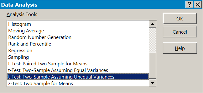
- Click the Data > Data Analysis button to open the Data Analysis dialogue window.

- Choose the t-test: Two-Sample Assuming Unequal Variances
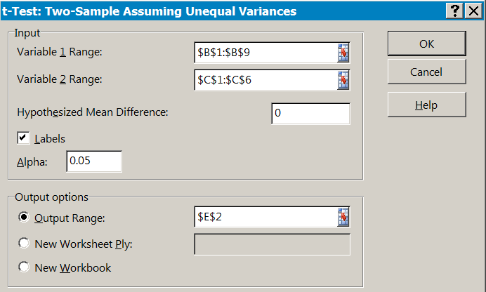
- Now select the appropriate data and fill in the boxes. Make sure you type a zero in the box labelled Hypothesized Mean Difference

- Choose the location to place the results. This can be a new workbook or worksheet. In the example above the results are placed in cell E2 of the existing sheet.
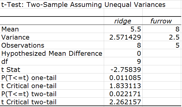
Now you just have to interpret the results!:

You can ignore the sign for the t Stat result, if the samples were in different column order the result would be the same value but with opposite sign.
Note that the df are shown as an integer and the exact value is always rounded upwards.
You want the two-tail results in most cases, which are in the last two rows.
Comments are closed.