Abundance-based dissimilarity metrics
Exercise 12.2.2.
Statistics for Ecologists (Edition 2) Exercise 12.2.2
In these notes you’ll see some of the more commonly used measures of dissimilarity used when you have abundance data.
Abundance-based dissimilarity metrics
Introduction
When your community data samples include abundance information (as opposed to simple presence-absence) you have a wider choice of metrics to use in calculating (dis)similarity. When you have presence-absence data you use the number of shared species (J) and the species richness of each sample (A & B). Measures of (dis)similarity obtained are therefore slightly “crude”.
When you have abundance data your measures of (dis)similarity are a bit more “refined” and you have the potential to pick up patterns in the data that you would otherwise not see using presence-absence data.
There are many metrics that you might use to explore (dis)similarity, in this exercise you’ll see four of the more commonly used ones:
- Bray-Curtis
- Canberra
- Manhattan (City Block)
- Euclidean
The exercise shows you how you can carry out the calculations using Excel (in the book you also see how to do this using R). You can get the sample spreadsheet here: Distance metrics.xlsx.
Notation
When you have presence-absence data you use the species richness of each sample, calling these values A and B. The number of shared species is designated J. When you have abundance data you use a slightly different notation. The abundance of an individual species is given as x. Now you are comparing two samples so you call one i and one j. Subscripts are used to differentiate the abundances between the two samples, so you get xi and xj.
Generally speaking it does not matter which sample is i and which is j.
You’ll also see the ∑ symbol (meaning sum, you add things together) and the vertical bars e.g. |x – y|, which indicate that you ignore any negative sign and simply use the magnitude of the result.
Bray-Curtis
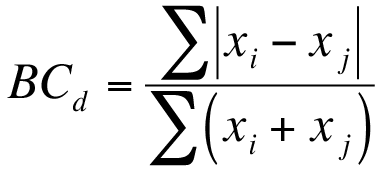
The Bray-Curtis metric uses two components: |xi – xj| and (xi + xj).
In the first case you subtract the abundance of one species in a sample from its counterpart in the other sample but ignore the sign. The second component is the abundance of a species in one sample added to the abundance of its counterpart in the second sample. If a species is absent, then its abundance should be recorded as 0 (zero).
The equation for the Bray-Curtis dissimilarity is shown below:

Bray-Curtis dissimilarity is easy to calculate in Excel but there are no shortcuts to working out the main components, |xi – xj| and (xi + xj).
You might have your data arranged in rows or columns; in the following example the data are in columns.
| Species | Si | Sj | |xi – xj| | (xi + xj) |
| Spp1 | 6 | 4 | 2 | 10 |
| Spp2 | 5 | 3 | 2 | 8 |
| Spp3 | 7 | 4 | 3 | 11 |
| Spp4 | 2 | 6 | 4 | 8 |
| Spp5 | 3 | 0 | 3 | 3 |
So, the 4th column is easily calculated by subtracting values in the 3rd column from the 2nd. Use the =ABS function to get the absolute value (i.e. ignore the sign). So for example the 4th data row would be 2 – 6 = -4 but the ABS function ignores the -.
The last column is even easier, as it is the sum of a value in the 2nd column with its counterpart in the 3rd column.
You don’t need to compute the sum of the 4th or 5th columns because your final calculation can do that in one go:
=SUM(column4) / SUM(column5)
You can use the mouse to highlight the values in the columns in place of the column4 and column5 items in the formula (which represent the cell ranges).
If you calculate the Bray-Curtis dissimilarity for these data, you get a result of 0.350.
If your data were arranged in rows the calculations are more or less the same (the spreadsheet shows both methods).
Canberra
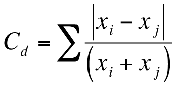
The Canberra dissimilarity uses the same components as Bray-Curtis but the components are summed differently:

In the Canberra metric each |xi – xj| result is divided by the corresponding (xi + xj) value.
In the following example the data are shown in rows but the calculations are more or less the same for data in columns (the spreadsheet shows both).
| Calc | Spp1 | Spp2 | Spp3 | Spp4 | Spp5 |
| Si | 6 | 5 | 7 | 2 | 3 |
| Sj | 4 | 3 | 4 | 6 | 0 |
| |xi – xj| | 2 | 2 | 3 | 4 | 3 |
| (xi + xj) | 10 | 8 | 11 | 8 | 3 |
This time you need to evaluate each |xi – xj| ÷ (xi + xj) then adding them together.
This means you need to work out 2/10 + 2/8 + 3/11 + 4/8 + 3/3 for the current example. There is no shortcut for this (obviously you will use the cell references) so when you have a lot of species the formula is quite long. You can get around this by making a new row (or column, depending how your data are arranged) for the |xi – xj| ÷ (xi + xj) values. You can then copy/paste the results and then do a final =SUM to get the Canberra distance.
In this case the result works out to be 2.223.
Manhattan (City Block)
The Manhattan (or City Block) dissimilarity uses the |xi – xj| component only.
This is the simplest dissimilarity metric to compute:

Manhattan (City Block) dissimilarity.
You can use the =ABS function to ignore any negative signs (and retain the value only). Then the =SUM funtion can simply total them to give the final result. In this case you get: 2 + 2 + 3 + 4 + 3 = 14.
As you can see, City Block dissimilarity is easy to work out using Excel.
Euclidean
The Euclidean dissimilarity metric uses a different component (xi – xj) from the other metrics.
Here the abundance of a species from one sample is subtracted from its counterpart in the other sample. Instead of ignoring the sign, the result is squared (which gives a positive value):

In this case you can use the =SUMXMY2 function to eliminate any intermediate calculation steps (although you can of course do those intermediate steps if you like).
=SUMXMY2(range1, range2)
What the function does is to take two ranges of cells, it subtracts one value from its counterpart in the other and squares the result, then gives the total. This is exactly what you want to calculate the Euclidean dissimilarity. All you need to do is to use =SUMXMY2 and then SQRT the result. You can of course do this in one formula.
The spreadsheet gives an example of the calculation in action for data in columns and in rows (there is little difference).
If you already had calculated |xi – xj| values, then you can use them. Simply square each one, add the squares together, there is a function to do that =SUMSQ. Then take a square root. You might as well use the =SUMXMY2 function!
In the example here the |xi – xj| values are 2, 2, 3, 4, 3.
Their squares would be 4, 4, 9, 16, 9 giving a total of 42.
The final Euclidean dissimilarity is √42 = 6.481.
Which metric to use?
Good question! There is no definite “correct” metric to use in most cases. As a rule of thumb you should use the metric that gives the best separation of samples. This runs a little counter to the idea in statistics that you decide on the proper test to apply before you begin. However, this is not a statistical “test” but a method of separating samples into meaningful groupings. Your distance values should be visualized using a dendrogram (see this exercise on drawing dendrograms in Excel). You choose the metric that gives the most useful results.
The choice of dissimilarity metrics is something that occasionally sparks low-level holy wars amongst ecologists. Hopefully you will use several and the results will all give broadly the same ecological meaning!
Example data and files
You can get examples from the book from the support pages. There are also some specific examples used for the exercises in addition to those shown in the book. You can also download the spreadsheet file Distance metrics.xlsx, which shows how to carry out the calculations using Excel.
Comments are closed.