Adjustment for tied ranks in the Kruskal-Wallis test
Exercise 10.2.b.
Statistics for Ecologists (Edition 2) Exercise 10.2.b
These notes are concerned with the Kruskal-Wallis test (Section 10.2). The notes show you how to adjust your test statistic when you have tied values, and so tied ranks.
Adjusting for tied ranks in the Kruskal-Wallis test
Introduction
The Kruskal-Wallis test is appropriate when you have non-parametric data and one predictor variable (Section 10.2). It is analogous to a one-way ANOVA but uses ranks of items in various groups to determine the likely significance.
When you have tied values, you will get tied ranks. In these circumstances you should apply a correction to your calculated test statistic. The notes show you how this can be done. The calculations are simple but in Excel it can be difficult to get the process “automated”. In R the kruskal.test() command computes the adjustment for you.
Calculating the adjustment factor
In order to correct for tied ranks you first need to know which values are tied. Then you need to know how many ties there are for each rank value. Finally, you’ll need to know how many replicates there are in the dataset.
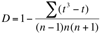
Once you’ve ascertained these things you can use the following formula to work out a correction, or adjustment, factor:

In the formula t is the number of ties for each rank value. For each value of t, you evaluate the t-cubed minus t part. This is then summed for all the tied values (values without ties can also be evaluated but 13 – 1 = 0). Once you have the numerator you work out the denominator using n, the number of replicates in the original dataset.
The final value of D is then 1 – your fraction.
Adjusting the KW test statistic
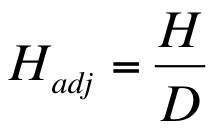
Once you have the value of D, the correction factor, you can use it to adjust the original Kruakal-Wallis test statistic (H).

Formula for adjustment of the Kruskal-Wallis statistic in the case of tied ranks.
The correction is simple: H/D.
You then use the Hadj value in place of the original to determine the final test significance (using critical values tables – see exercise 10.2a).
Example data
Have a look at the correction in action using the following example:
Example data. Three non-parametric samples for use in Kruskal-Wallis test.
| Upper | Mid | Lower |
| 3 | 4 | 11 |
| 4 | 3 | 12 |
| 5 | 7 | 9 |
| 9 | 9 | 10 |
| 8 | 11 | 11 |
| 10 | ||
| 9 |
Here there are three samples and you can see that there are tied values, so you know there will be tied ranks.
Example ranks
The first step is to evaluate the ranks. Each value is replaced by its rank in the overall dataset.
Sample data shown as ranks instead of original values. Samples are combined for ranking.
| Upper | Mid | Lower |
| 1.5 | 3.5 | 15 |
| 3.5 | 1.5 | 17 |
| 5 | 6 | 9.5 |
| 9.5 | 9.5 | 12.5 |
| 7 | 15 | 15 |
| 12.5 | ||
| 9.5 |
The Kruskal-Wallis test looks at the sum of the ranks from each sample. If the ∑rank is different between samples there is a good chance that differences are statistically significant. If the ∑rank are close, then differences are less likely to be significant.
In this example the rank sums are:
Rank sums for three samples.
| Upper | Mid | Lower |
| 48.5 | 35.5 | 69 |
You can now calculate the Kruskal-Wallis test statistic, H.
Original H value
Once you have the rank sums you can compute the Kruskal-Wallis test statistic:

Formula for calculating the Kruskal-Wallis statistic for non-parametric samples.
The Kruskal–Wallis formula looks pretty horrendous but actually it is not that bad. The numbers 12 and 3 are constants. Uppercase N is the total number of observations. The R refers to the ranks of the observations in each sample and n is the number of observations per sample.
In the example the final value of the Kruskal-Wallis statistic works out to be H = 6.403.
Tied ranks
The formula for working out the correction factor was given earlier. You need to work out, for each rank value, the number of repeats.
It is not easy to do this “automatically” using Excel. There are ways you could make a template to evaluate the ties for you but it is complicated. Since you can do it using a bit of copy and paste, this is what you’ll see here.
Start by assembling the ranks into a single column. This means a bit of copy and paste but you’ll probably need to use Paste Special to place the Values only.

When you paste the ranks you only want the numbers and don’t want the formula (which would give an error).
Once you have the column of ranks you can simply re-arrange them in ascending order (use the Home > Sort & Filter button or the Data > Sort button). In the following table the second column shows the sorted ranks (you don’t need to make a second column, I have done this to show the effect).
Rearranging ranked data to make calculation of tied ranks easier.
| Rnk | Ord | Ties | T3-T |
| 1.5 | 1.5 | ||
| 3.5 | 1.5 | 2 | 6 |
| 5 | 3.5 | ||
| 9.5 | 3.5 | 2 | 6 |
| 7 | 5 | ||
| 12.5 | 6 | ||
| 9.5 | 7 | ||
| 48.5 | 9.5 | ||
| 3.5 | 9.5 | ||
| 1.5 | 9.5 | ||
| 6 | 9.5 | 4 | 60 |
| 9.5 | 12.5 | ||
| 15 | 12.5 | 2 | 6 |
| 17 | 15 | ||
| 9.5 | 15 | ||
| 12.5 | 15 | 3 | 24 |
| 15 | 17 | ||
| 15 | 48.5 |
Once you have the ranks in order it is easy to work out the number of repeats by inspection. You can simply fill in the values as you work down the column. In the preceding table the 3rd column shows the tied rank repeats. So, for example the rank 1.5 is repeated 2 times. The rank 9.5 has 4 repeats.
The final column shows the T3 – T values. In other words, you take the number of repeats and cube it, then subtract the number of repeats.
Once you have these values you can sum them to get an overall value, in this case 102.
Final H adjustment
Once you have your final sum of T3 -3 values you can work out the value of D using the formula given earlier. You need to know the total number of replicates in the original dataset (in this case 17).
The final value of D works out at: 0.9792.
The adjusted H value is then H/D = 6.403 / 0.9792 = 6.540.
You can now use the adjusted H-value to compare to critical value tables (see exercise 10.2a) to see if your result is statistically significant.
Comments are closed.