The new book An Introduction to R: Data Analysis and Visualisation is now in print as of May 2023.
The book is published by Pelagic Publishing. Buy the Book here.

The new book An Introduction to R: Data Analysis and Visualisation is now in print as of May 2023.
The book is published by Pelagic Publishing. Buy the Book here.

Matrix math operations using R are easy to conduct using basic math operators such as + - * and /. Generally speaking the matrix objects you perform math on must be the same dimensions (that is conformable) as each other but there are exceptions.
There are two kinds of matrix math:
matrix simply as a series of values.In the first case you can use R to carry out regular mathematical operations on a matrix (that is a 2-dimensional array). In the second case you use R to conduct “proper” matrix math.
This article is not intended to be a detailed treatise on matrix math; think of it more as a rough guide to possibilities. If matrix math is what you need then this might help point you in the right direction.
Here are some of the topics covered:
Matrix math operations using R can be fairly simple. In the “simple” case you can use a matrix with basic math operators.
The “simplest” situation is where you have matrix objects that have the same dimensions.
x <- matrix(c(1,1, 3,0, 1,0), ncol = 3))
y <- matrix(c(0,7, 0,5, 5,0), ncol = 3)
x ; y

     [,1] [,2] [,3]
[1,]    1    3    1
[2,]    1    0    0

     [,1] [,2] [,3]
[1,]    0    0    5
[2,]    7    5    0
The regular math operators with deal with the calculations:
x + y
     [,1] [,2] [,3]
[1,]    1    3    6
[2,]    8    5    0

x * y
     [,1] [,2] [,3]
[1,]    0    0    5
[2,]    7    0    0

x / y
          [,1] [,2] [,3]
[1,]       Inf  Inf  0.2
[2,] 0.1428571    0  NaN

x - y
     [,1] [,2] [,3]
[1,]    1    3   -4
[2,]   -6   -5    0
In the preceding example 2 matrix objects were used but there is no reason why you cannot have more, as long as they all have the same dimensions.
If you have a matrix you can also use the basic operators with a single value:
x * 4.5
     [,1] [,2] [,3]
[1,]  4.5 13.5  4.5
[2,]  4.5  0.0  0.0

y / 2
     [,1] [,2] [,3]
[1,]  0.0  0.0  2.5
[2,]  3.5  2.5  0.0
You can think of a matrix as a vector of values that happens to be split into rows and columns. This means that you can carry out math operations with a matrix and a vector of values, as long as the recursive process “fits” (i.e. is conformable).
In practical terms you can carry out a math operation between a matrix and a vector if the length of the matrix is divisible by the length of the vector exactly (i.e. producing an integer).
In the following example, the matrix has 6 elements and therefore any vector would have to contain 1, 2, or 3 elements. If your vector is too long it is truncated and you get a warning.
x
     [,1] [,2] [,3]
[1,]    1    3    1
[2,]    1    0    0

length(x)
[1] 6

x * 2:4
     [,1] [,2] [,3]
[1,]    2   12    3
[2,]    3    0    0

# Long vectors are truncated with a warning
x + 1:4
     [,1] [,2] [,3]
[1,]    2    6    2
[2,]    3    4    2

Warning message:
In x + 1:4 :
  longer object length is not a multiple of shorter object length
It can help to see your matrix as a vector:
c(x)
[1] 1 1 3 0 1 0

c(x) * 2:4
[1]  2  3 12  0  3  0

c(x) + 1:4
[1] 2 3 6 4 2 2

Warning message:
In c(x) + 1:4 :
  longer object length is not a multiple of shorter object length
Note that c(x) was used in the example but as.numeric(x) would also work.
Many math functions that can operate on a vector will be able to work with a matrix. For example:
xx
     [,1] [,2] [,3]
[1,]    1    2    3
[2,]    4    5    6

log(xx)
         [,1]      [,2]     [,3]
[1,] 0.000000 0.6931472 1.098612
[2,] 1.386294 1.6094379 1.791759

cos(xx)
           [,1]       [,2]       [,3]
[1,]  0.5403023 -0.4161468 -0.9899925
[2,] -0.6536436  0.2836622  0.9601703

sqrt(xx)
     [,1]     [,2]     [,3]
[1,]    1 1.414214 1.732051
[2,]    2 2.236068 2.449490
When you have two matrix objects of different dimensions you get an error. This example shows a single dimension matrix:
yy <- matrix(c(40,100), ncol = 1)
yy
     [,1]
[1,]   10
[2,]  100

x * yy
Error in x * yy : non-conformable arrays
In this case the matrix can be converted to a vector resulting in 2 elements. This is divisible by the number of elements in the first matrix and permits matrix math:
x * c(yy)
     [,1] [,2] [,3]
[1,]   10   30   10
[2,]  100    0    0

x + c(yy)
     [,1] [,2] [,3]
[1,]   11   13   11
[2,]  101  100  100
There are other solutions for this case:
xx * c(yy)
sweep(xx, 1, yy, `*`)
apply(xx, 2, function(x) x * yy)
xx * yy[,1]
xx * yy[row(xx),]
These solutions work for any of the math operators + - * and /.
Matrix math operations using R involve more than just simple math. In mathematics matrix math is a substantial topic. Using R you can carry out various matrix math computations. These include:
%*%outer() and %o%kronecker() and %x%diag()eigen()svd()chol()qr()det()crossprod() and tcrossprod()t()upper.tri() and lower.tri()row() and col()Standard matrix multiplication (or inner product) is a way to multiply two matrix objects. You use the %*% operator in Rto execute the math.
X %*% Y
In general if the number of columns of the first matrix equals the number of rows of the second matrix then you should be able to use the matrix-math operator %*% to multiply:
X <- matrix(c(2,7,4,8,5,9), ncol = 3)
Y <- matrix(c(1,3,4,6,1,2), ncol = 2)

X ; Y
     [,1] [,2] [,3]
[1,]    2    4    5
[2,]    7    8    9

     [,1] [,2]
[1,]    1    6
[2,]    3    1
[3,]    4    2

X %*% Y
     [,1] [,2]
[1,]   34   26
[2,]   67   68
The outer product is a matrix operation that takes a matrix (or vector or array) and applies a function to it, with a second matrix (or a vector or array) as an argument. There are two options in R:
outer(X, Y, FUN = "*", ...)
X %o% Y
The outer() command allows any maths function, with the default being *. Essentially X and Y are the main arguments (you can pass additional parameters too). The %o% operator (the letter o) is a convenience function for multiply (i.e. FUN = "*") so you end up specifying X multiplied by Y.
Use two vectors and the result is a matrix with dimensions determined by the length of the vectors:
outer(1:3, 1:3)
     [,1] [,2] [,3]
[1,]    1    2    3
[2,]    2    4    6
[3,]    3    6    9
You can use different function, and use Y as a parameter passed to FUN, in the following example Y specifies the base for the log:
m
     [,1] [,2]
[1,]    5    1
[2,]    1    3

outer(m, Y = 2, FUN = log)
, , 1

         [,1]     [,2]
[1,] 2.321928 0.000000
[2,] 0.000000 1.584963
Essentially what happens is that the second matrix is converted to a vector and this is “applied” to the first matrix using the function specified. Each element of the second matrix is applied in turn, and the result is an array with multiple dimensions. In the following example the first matrix is 2×2 and so is the second, so the result has dimensions of: 2, 2, 2, 2
A
     [,1] [,2]
[1,]    4   -1
[2,]    1    3

m
     [,1] [,2]
[1,]    5    1
[2,]    1    3

outer(A, m, FUN = "+")
, , 1, 1

     [,1] [,2]
[1,]    9    4
[2,]    6    8

, , 2, 1

     [,1] [,2]
[1,]    5    0
[2,]    2    4

, , 1, 2

     [,1] [,2]
[1,]    5    0
[2,]    2    4

, , 2, 2

     [,1] [,2]
[1,]    7    2
[2,]    4    6

# Get identical result using a vector
outer(A, c(5,1,1,3), FUN = "+")
The Kronecker matrix product is similar to the outer product but the result is a single array with dimensions equal to dim(X) x dim(Y).
kronecker(X, Y, FUN = "*", ...)
X %x% Y
The kronecker() command allows any function to be used, whist the alias %x% is for multiply (i.e. FUN = "*").
m
     [,1] [,2]
[1,]    5    1
[2,]    1    3

m %x% 2
     [,1] [,2]
[1,]   10    2
[2,]    2    6
When your second array has >1 dimension, the result has dimensions equal to dim(X) x dim(Y).
kronecker(m, 2:3, FUN = "+")
     [,1] [,2]
[1,]    7    3
[2,]    8    4
[3,]    3    5
[4,]    4    6

xx
     [,1] [,2] [,3]
[1,]    1    2    3
[2,]    4    5    6

yy
     [,1]
[1,]   10
[2,]  100

kronecker(xx, yy)
     [,1] [,2] [,3]
[1,]   10   20   30
[2,]  100  200  300
[3,]   40   50   60
[4,]  400  500  600
A matrix diagonal is more or less what it sounds like! Matrix diagonals are used in various branches of matrix math. In Ryou can use the diag() function to extract or create matrix diagonals.
diag(x = 1, nrow, ncol, names = TRUE)
diag(x) <- value
There are 4 main uses for diag():
x (a matrix).matrix by specifying nrow.matrix by specifying x as a scalar.matrix with specified diagonals.You can also assign diagonal values to an existing matrix.
To extract the diagonals from a matrix you simply specify the matrix:
C
     [,1] [,2] [,3]
[1,]    3    1   -5
[2,]    2    0    4
[3,]    1    6    3

diag(C)
[1] 3 0 3
If the matrix is not square you get the diagonals starting from the top-left:
E
     [,1] [,2] [,3]
[1,]   -3    2    0
[2,]    0    5   -1

diag(E)
[1] -3  5
If you omit x and specify nrow you will return an identity matrix, that is one where the diagonals are 1 and the other elements are 0. You may also give ncol to create a non-square matrix (note that ncol may be larger or smaller than nrow):
diag(nrow = 4)
     [,1] [,2] [,3] [,4]
[1,]    1    0    0    0
[2,]    0    1    0    0
[3,]    0    0    1    0
[4,]    0    0    0    1

diag(nrow = 4, ncol = 3)
     [,1] [,2] [,3]
[1,]    1    0    0
[2,]    0    1    0
[3,]    0    0    1
[4,]    0    0    0

diag(nrow = 4, ncol = 6)
     [,1] [,2] [,3] [,4] [,5] [,6]
[1,]    1    0    0    0    0    0
[2,]    0    1    0    0    0    0
[3,]    0    0    1    0    0    0
[4,]    0    0    0    1    0    0
If you specify x as a scalar (single value) you return an identity matrix with diagonals of 1 and with dimensions (nrow, ncol) set to the of the scalar:
diag(4)
     [,1] [,2] [,3] [,4]
[1,]    1    0    0    0
[2,]    0    1    0    0
[3,]    0    0    1    0
[4,]    0    0    0    1
If you specify x as a vector you will return a matrix where the diagonals are the values in x and the other elements are 0:
diag(x = c(3,4,2,6))
     [,1] [,2] [,3] [,4]
[1,]    3    0    0    0
[2,]    0    4    0    0
[3,]    0    0    2    0
[4,]    0    0    0    6
You can set the diagonals for an existing matrix by assigning values:
mm
     [,1] [,2]
[1,]    8    1
[2,]    1    9

diag(mm) <- 100
mm
     [,1] [,2]
[1,]  100    1
[2,]    1  100

diag(mm) <- c(6,3)
mm
     [,1] [,2]
[1,]    6    1
[2,]    1    3

CC
     [,1] [,2] [,3]
[1,]    3    1   -5
[2,]    2    0    4
[3,]    1    6    3

diag(CC) <- c(99, 999)
Error in `diag<-`(`*tmp*`, value = c(99, 999)) :
  replacement diagonal has wrong length
Note:
Spectral decomposition of a matrix produces eigenvalues and eigenvectors. These values are used often in linear algebra and various branches of mathematics.
The R function eigen() can compute the eigenvalues and eigenvectors of a (square) matrix.
eigen(x, symmetric, only.values = FALSE)
The eigen() function only works on square matrix objects.
The symmetric parameter allows you to specify TRUE to force the calculations to use only the lower triangle, when you have symmetrical matrix objects. If you leave this to the default then the function checks to see if the values are symmetric.
The only.values parameter can be set to TRUE to return only the eigenvalues.
m
     [,1] [,2]
[1,]    5    1
[2,]    1    3

eigen(m)
eigen() decomposition
$values
[1] 5.414214 2.585786

$vectors
           [,1]       [,2]
[1,] -0.9238795  0.3826834
[2,] -0.3826834 -0.9238795
If you have negative values you’ll return complex values:
M
     [,1] [,2]
[1,]    5   -2
[2,]    2    4

eigen(M)
eigen() decomposition
$values
[1] 4.5+1.936492i 4.5-1.936492i

$vectors
                     [,1]                 [,2]
[1,] 0.7071068+0.0000000i 0.7071068+0.0000000i
[2,] 0.1767767-0.6846532i 0.1767767+0.6846532i
Singular value decomposition of a matrix is important in many statistical routines. SVD is a kind of factorisation of a matrix and is carried out in R with the svd() function:
svd(x, nu = min(n, p), nv = min(n, p))
In the svd() function:
x is a matrixnu is the number of left singular vectors to computenv is the number of right singular vectors to computeThe svd() function returns a result with several components:
$d a vector of singular values in descending order.$u a matrix of left singular vectors.$v a matrix of right singular vectors.C
[,1] [,2] [,3]
[1,] 3 1 -5
[2,] 2 0 4
[3,] 1 6 3
svd(C)
$d
[1] 7.620874 5.810848 3.025941
$u
[,1] [,2] [,3]
[1,] -0.4710376 -0.7804341 -0.4111522
[2,] 0.4517527 0.1869132 -0.8723434
[3,] 0.7576563 -0.5966457 0.2645201
$v
[,1] [,2] [,3]
[1,] 0.03254861 -0.4412646 -0.8967866
[2,] 0.53470246 -0.7503738 0.3886290
[3,] 0.84441333 0.4921633 -0.2115217
You can use the nu and nv arguments to reduce (to 0 if you like) the number of left and/or right singular vectors.
VADeaths
      Rural Male Rural Female Urban Male Urban Female
50-54       11.7          8.7       15.4          8.4
55-59       18.1         11.7       24.3         13.6
60-64       26.9         20.3       37.0         19.3
65-69       41.0         30.9       54.6         35.1
70-74       66.0         54.3       71.1         50.0

svd(VADeaths, nu = 2, nv = 2)
$d
[1] 161.967972  10.037542   3.212076   1.194284

$u
           [,1]       [,2]
[1,] -0.1404491 -0.1476512
[2,] -0.2161352 -0.3623160
[3,] -0.3297674 -0.4373676
[4,] -0.5099065 -0.4819224
[5,] -0.7515374  0.6506817

$v
           [,1]       [,2]
[1,] -0.5243856  0.3123820
[2,] -0.4137210  0.6015805
[3,] -0.6229108 -0.7282861
[4,] -0.4072306  0.1005871
Compute the Choleski (Cholesky) factorization of a real symmetric positive-definite square matrix using the chol()function. It is a kind of optimisation that can be used in various mathematical problems.
chol(x, pivot = FALSE, tol = -1, ...)
In chol():
x is a matrix, which should be positive and symmetric, (i.e. square).pivot can be set to TRUE in some cases where the matrix is semi-positive definite.tol is used to set a tolerance when pivot = TRUE.How to tell if a matrix is positive definite, or positive semi-definite?
matrix is symmetric if nrow = ncol, in other words, square. In addition the transposed matrix must be the same as the original.matrix is positive definite.0 and the others positive then the matrix is positive semi-definite.You can check the eigenvalues with eigen(x).
m
     [,1] [,2]
[1,]    5    1
[2,]    1    3

# Check matrix is positive definite
eigen(m)$val
[1] 5.414214 2.585786

# Check that matrix is symmetric
identical(m, t(m))
[1] TRUE

chol(m)
         [,1]      [,2]
[1,] 2.236068 0.4472136
[2,] 0.000000 1.6733201

A
     [,1] [,2]
[1,]    4   -1
[2,]    1    3

# Check matrix (it is complex but is +ve definite)
eigen(A)$val
[1] 3.5+0.866025i 3.5-0.866025i

# Check if matrix is symmetric
identical(A, t(A))
[1] FALSE

# chol() will return a result as it does not check symmetry!
If you have an eigenvalue of 0 (with the others >0) then your matrix is positive semi-definite. You can perform Cholensky decomposition with chol() but need to use pivot = TRUE as an argument.
im <- matrix(c(1,-1, -1,1), ncol = 2)

im
     [,1] [,2]
[1,]    1   -1
[2,]   -1    1

# matrix is +ve semi-definite
eigen(im)$val
[1] 2 0

# Check symmetric
identical(im, t(im))
[1] TRUE

chol(im)
Error in chol.default(im) :
  the leading minor of order 2 is not positive definite

# Need to use pivot = TRUE
chol(im, pivot = TRUE)
     [,1] [,2]
[1,]    1   -1
[2,]    0    0
attr(,"pivot")
[1] 1 2
attr(,"rank")
[1] 1
Warning message:
In chol.default(im, pivot = TRUE) :
  the matrix is either rank-deficient or indefinite
Note that you still get a warning!
The eigenvalues need to be >0 but there is a tolerance:
mat <- matrix(c(4,12,-16, 12,37,-43, -16,-43,98), ncol = 3)
mat
     [,1] [,2] [,3]
[1,]    4   12  -16
[2,]   12   37  -43
[3,]  -16  -43   98

# Eigenvalues all >0 (just)
eigen(mat)$val
[1] 123.47723179  15.50396323   0.01880498

# Check symmetry
identical(mat, t(mat))
[1] TRUE

chol(mat)
     [,1] [,2] [,3]
[1,]    2    6   -8
[2,]    0    1    5
[3,]    0    0    3

a <- matrix(c(2,3,1,11, 3,9,3,30, 1,3,1,10, 11,30,10,101))
a
     [,1] [,2] [,3] [,4]
[1,]    2    3    1   11
[2,]    3    9    3   30
[3,]    1    3    1   10
[4,]   11   30   10  101

# Very small eigenvalue registers as effectively 0
eigen(a)$val
[1] 1.120990e+02 9.009892e-01 1.681988e-14 1.831868e-15

# Check symmetry
identical(a, t(a))
[1] TRUE

chol(a)
Error in chol.default(a) :
  the leading minor of order 3 is not positive definite
If you try to use pivot = TRUE on a matrix that is not positive (i.e. non-negative definite), you’ll get a result with a warning. However, the result will be meaningless!
# Negative definite i.e. not non-negative definite
b <- matrix(c(5,-5,-5,3), 2, 2)
b
     [,1] [,2]
[1,]    5   -5
[2,]   -5    3

# check symmetry -- okay
identical(b, t(b))
[1] TRUE

# negative eigenvalues, so no +ve
eigen(b)$val
[1]  9.09902 -1.09902

# pivot = TRUE runs but result is meaningless!
#.. not shown
QR decomposition is used in many statistical methods, especially in regression. The qr() function carries out the calculations.
qr(x, tol = 1e-07 , LAPACK = FALSE, ...)
In qr():
x is a matrix to be decomposed.tol is a tolerance used for detecting linear dependencies (you probably won’t need to tinker with this).LAPACK is which QR algorithm to use, the default uses LINPACK.The result of qr() is an object with various components:
C
     [,1] [,2] [,3]
[1,]    3    1   -5
[2,]    2    0    4
[3,]    1    6    3

qr(C)
$qr
           [,1]      [,2]     [,3]
[1,] -3.7416574 -2.405351 1.069045
[2,]  0.5345225  5.586975 2.787095
[3,]  0.2672612 -0.983516 6.410089

$rank
[1] 3

$qraux
[1] 1.801784 1.180821 6.410089

$pivot
[1] 1 2 3

attr(,"class")
[1] "qr"
QR decomposition is a potentially large topic, which there is not space for here! In addition to the qr() function there are various helper functions. See the help entry in qr() for more information about those.
You can calculate the of a square matrix using the det() function. A square matrix is one where nrow = ncol but it doesn’t have to be symmetrical (where x = t(x)).
det(x)
determinant(x, logarithm = TRUE)
The det() function returns the determinant. The determinant() function returns the modulus of the determinant and the sign. The default for determinant() is to return the log of the determinant.
A
     [,1] [,2]
[1,]    4   -1
[2,]    1    3

# Matrix is square but no matter that it is not symmetric
identical(A, t(A))
[1] FALSE

det(A)
[1] 13

determinant(A)
$modulus
[1] 2.564949
attr(,"logarithm")
[1] TRUE

$sign
[1] 1

attr(,"class")
[1] "det"

determinant(A, logarithm = FALSE)
$modulus
[1] 13
attr(,"logarithm")
[1] FALSE

$sign
[1] 1

attr(,"class")
[1] "det"
Note that the logarithm argument cannot be abbreviated.
Cross products are where you multiply two matrix objects (inner product), but one is transposed. The R functions crossprod() and tcrossprod() can carry out the calculations.
crossprod(x, y = NULL)
tcrossprod(x, y = NULL)
You specify at least one matrix object x. Object y is optional, if not specified x is used. These functions are essentially equivalent to:
t(x) %*% y for crossprod()x %*% t(y) for tcrossprod()b
[,1] [,2]
[1,] 5 -5
[2,] -5 3
crossprod(b)
[,1] [,2]
[1,] 50 -40
[2,] -40 34
B
[,1] [,2]
[1,] 1 3
[2,] -2 -4
[3,] 2 0
D
[,1]
[1,] 3
[2,] 2
[3,] -2
crossprod(B, D)
[,1]
[1,] -5
[2,] 1
You get an error if the dimensions are “wrong”:
A
     [,1] [,2]
[1,]    4   -1
[2,]    1    3

D
     [,1]
[1,]    3
[2,]    2
[3,]   -2

crossprod(A, D)
Error in crossprod(A, D) : non-conformable arguments
If you specify a vector it will be “converted” to a one-column or one-row matrix:
tcrossprod(1:4)
     [,1] [,2] [,3] [,4]
[1,]    1    2    3    4
[2,]    2    4    6    8
[3,]    3    6    9   12
[4,]    4    8   12   16
There are various other tools that you can use with matrix objects:
Perhaps the simplest matrix operation is to transpose, that is switch the rows and columns. You can carry out matrixtransposition using the t() function.
t(x)
Example: transpose matrix objects
x
     [,1] [,2] [,3]
[1,]    1    3    1
[2,]    1    0    0

t(x)
     [,1] [,2]
[1,]    1    1
[2,]    3    0
[3,]    1    0

D
     [,1]
[1,]    3
[2,]    2
[3,]   -2

t(D)
     [,1] [,2] [,3]
[1,]    3    2   -2
You can “see” the upper or lower triangles of a matrix (or any 2-D object) using upper.tri() and lower.tri()functions. These give you a logical matrix the same size as the original, i.e. TRUE or FALSE values.
upper.tri(x, diag = FALSE)
lower.tri(x, diag = FALSE)
You can optionally set diag = TRUE to return the diagonals as TRUE.
A
     [,1] [,2]
[1,]    4   -1
[2,]    1    3

upper.tri(A)
      [,1]  [,2]
[1,] FALSE  TRUE
[2,] FALSE FALSE

B
     [,1] [,2]
[1,]    1    3
[2,]   -2   -4
[3,]    2    0

lower.tri(B, diag = TRUE)
     [,1]  [,2]
[1,] TRUE FALSE
[2,] TRUE  TRUE
[3,] TRUE  TRUE
You can produce a matrix of integer values based on their position in a matrix object (or similar 2-D object). The row() and col() functions operate over rows and columns respectively.
row(x, as.factor = FALSE)
.row(dim)

col(x, as.factor = FALSE)
.col(dim)
Essentially you provide a template object and the functions return a new object with the appropriate values.
C
     [,1] [,2] [,3]
[1,]    3    1   -5
[2,]    2    0    4
[3,]    1    6    3

row(C)
     [,1] [,2] [,3]
[1,]    1    1    1
[2,]    2    2    2
[3,]    3    3    3
If you specify the argument as.factor you can get the result stored as a factor rather than a regular numeric.
E
     [,1] [,2] [,3]
[1,]   -3    2    0
[2,]    0    5   -1

col(E, as.factor = TRUE)
     [,1] [,2] [,3]
[1,] 1    2    3
[2,] 1    2    3
Levels: 1 2 3
There are alternative versions .row() and .col(), which take a vector argument, giving the dimensions of the matrixfor which the indices are required.
.row(dim = c(3, 5))
     [,1] [,2] [,3] [,4] [,5]
[1,]    1    1    1    1    1
[2,]    2    2    2    2    2
[3,]    3    3    3    3    3
The topic of matrix math is extensive! This article is not intended to be an exhaustive thesis on the subject but more of an introduction to some of the R tools that you can use to carry out matrix math, and other operations.
This article is partly in support of my book An Introduction to R see the publications page for more information.
An Introduction to R will be published by Pelagic Publishing. See all my books at Pelagic Publishing.
For more articles visit the Tips and Tricks page and look for the various categories or use the search box.
See also the Knowledge Base where there are other topics related to R and data science.
Look at our other books on the Publications Page.
Visit our other site at GardenersOwn for a more ecological matters.

Association plots in R. An association plot draws the results of an association test by charting the Pearson Residuals.
Association plots in R are drawn using assocplot()
assocplot(x, col = c("black", "red"), space = 0.3,
          main = NULL, xlab = NULL, ylab = NULL)
| Parameter | Explanation |
|---|---|
x |
the data, usually a numeric matrix. |
col |
colors for positive and negative associations. |
space |
amount of space between the bars, as a fraction of average bar height and width (default = 0.3). |
main, xlab, ylab |
title annotations. |
Essentially you need a 2-dimensional matrix to use assocplot():
VADeaths
      Rural Male Rural Female Urban Male Urban Female
50-54       11.7          8.7       15.4          8.4
55-59       18.1         11.7       24.3         13.6
60-64       26.9         20.3       37.0         19.3
65-69       41.0         30.9       54.6         35.1
70-74       66.0         54.3       71.1         50.0
Apart from the titles, the only graphical parameter you can alter directly is col, to alter the positive and negative bar colors:
assocplot(VADeaths, col = c("lightblue", "pink"),
	  xlab = "Age class", ylab = "Driver actegory")

Basic association plot using custom color for positive and negative bars
If you want to alter the general appearance of your association plot you’ll need to set the appropriate graphical parameters using par() before using assocplot():
opar <- par(las = 1, cex = 0.8, mar = c(5,7,2,1))

assocplot(VADeaths, col = c("blue", "tomato"),
          space = 0.05, xlab = "Age class")
title(ylab = "Driver category", line = 6)

par(opar)
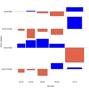
Custom graphical parameters have to be applied using par() before using assocplot()
In the preceding example the margins were widened to allow the labels to “fit”. Note also how title() was used to place the y-axis annotation on an outer line.
Essentially you need a 2D matrix for assocplot() to make an association plot in R. If you have something else you need to coerce it to the correct form.
Here are some options:
data.frame use as.matrix() to alter the form.table use x[r, c, n, ...] to “pick out” the appropriate 2D sub-table or..table use margin.table to “collapse” a table and combine across the margins you want.# 3D table
HairEyeColor
, , Sex = Male

       Eye
Hair    Brown Blue Hazel Green
  Black    32   11    10     3
  Brown    53   50    25    15
  Red      10   10     7     7
  Blond     3   30     5     8

, , Sex = Female

       Eye
Hair    Brown Blue Hazel Green
  Black    36    9     5     2
  Brown    66   34    29    14
  Red      16    7     7     7
  Blond     4   64     5     8
# Choose "Male"
HairEyeColor[,,1]
       Eye
Hair    Brown Blue Hazel Green
  Black    32   11    10     3
  Brown    53   50    25    15
  Red      10   10     7     7
  Blond     3   30     5     8
# Combine "Male" and "Female"
margin.table(HairEyeColor, margin = c(1,2))
       Eye
Hair    Brown Blue Hazel Green
  Black    68   20    15     5
  Brown   119   84    54    29
  Red      26   17    14    14
  Blond     7   94    10    16
# Combine "Eye"
margin.table(HairEyeColor, margin = c(1,3))
       Sex
Hair    Male Female
  Black   56     52
  Brown  143    143
  Red     34     37
  Blond   46     81
The assocplot() function is not the only was to draw an association plot using R. You could run a chisq.test() and extract the Pearson residuals $residuals, which you then plot using barplot().
X <- chisq.test(VADeaths)
X$residuals
         Rural Male Rural Female Urban Male Urban Female
50-54 -0.0001229145  -0.09956533  0.2454344  -0.21106734
55-59  0.0422284686  -0.56107962  0.4550546  -0.06391943
60-64 -0.0951496863  -0.16808112  0.5368919  -0.40335827
65-69 -0.2718462679  -0.34870589  0.2349807   0.36003546
70-74  0.2624133483   0.73510055 -0.8898149   0.09370444
barplot(X$residuals, beside = TRUE, col = cm.colors(5),
        ylim = c(-1,1), legend = TRUE,
	args.legend = list(x = "top", bty = "n", ncol = 5))
title(ylab = "Pearson residuals", xlab = "Category")
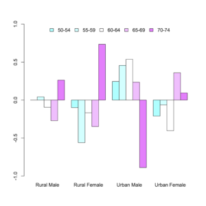
Alternative to assocplot() is to use barplot() on the Pearson residuals
To get multiple rows, with a separate mini-plot for each row you would need to set-up par(mfrow = c(rows, cols)).
There are potential advantages to this method, for example you can add horizontal lines at +/- 2 to show the “significance band”. However, it is also somewhat more involved!
This article is partly in support of my book An Introduction to R see the publications page for more information.

Conditional density plots in R — how to draw a conditional density plot using R. A conditional density plot shows the density of a sample split into groups.
Use cdplot() to draw a conditional density plot using R.
cdplot(x, y,
       plot = TRUE, tol.ylab = 0.05, ylevels = NULL,
       bw = "nrd0", n = 512, from = NULL, to = NULL,
       col = NULL, border = 1, main = "", xlab = NULL, ylab = NULL,
       yaxlabels = NULL, xlim = NULL, ylim = c(0, 1), ...)
There are many potential parameters for cdplot() but the most helpful are:
| Parameter | Explanation |
|---|---|
x, y |
the data, specify x and y or use a formula. In any event y should be a factor and x a numeric |
ylevels |
the order of the variables to be plotted |
yaxlabels |
labels for axis annotation |
bw, n, from, to, ... |
arguments to pass to density |
There are several arguments related to the density() function, which in most cases you’ll never need to alter.
A basic plot requires a factor variable and a numeric:
cdplot(tension ~ breaks, data = warpbreaks)
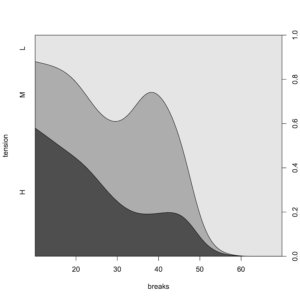
A conditional density plot
You can use the ylevels argument to alter the order of the plotting of a cdplot():
cdplot(tension ~ breaks, data = warpbreaks, ylevels = 3:1)
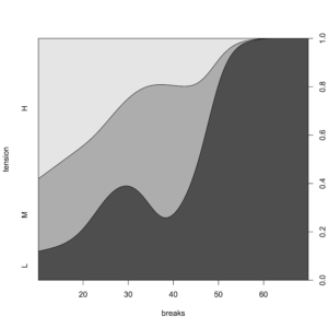
Use the ylevels argument to change the order of a conditional density plot
Give customized names to the factor levels via the yaxlabels argument:
cdplot(group ~ weight, data = PlantGrowth,
       yaxlabels = c("Control", "Treatment-1", "Treatment-2"))
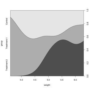
Custom factor labels via yaxlabels argument in cdplot
Only some of the general graphical parameters can be changed in cdplot(), as in the following example.
Use graphical parameters col and border to alter the appearance:
cdplot(spray ~ count, data = InsectSprays,
       col = cm.colors(6), border = "blue")
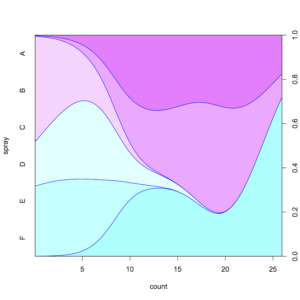
Basic graphical parameters col and border used to alter a cdplot
If you want to change any other graphical parameters you’ll need to call par() first:
opar <- par(las = 1, cex = 0.8, mar = c(5,7,2,3))

cdplot(feed ~ weight, data = chickwts, ylab = "")
title(ylab = "feed", line = 5)

par(opar)
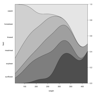
Use par() to set graphical parameters (other than col, border) in a cdplot
In the preceding example the margins were altered to allow the annotations to “fit”. In the title the annotation was shifted outwards.
This article is partly in support of my book An Introduction to R see the publications page for more information.

A spine plot is similar to a mosaic plot and stacked bar chart. Use spineplot() function to draw spine plots using R. There are quite a number of potential arguments you can use:
spineplot(x, y = NULL,
          breaks = NULL, tol.ylab = 0.05, off = NULL,
          ylevels = NULL, col = NULL,
          main = "", xlab = NULL, ylab = NULL,
          xaxlabels = NULL, yaxlabels = NULL,
          xlim = NULL, ylim = c(0, 1), axes = TRUE, ...)
The major parameters are:
| Parameter | Result |
|---|---|
x |
data (x,y) or formula y~x |
breaks |
passed to hist() |
off |
space between bars |
ylevels |
order of levels in x |
col |
colors |
xaxlabels |
labels for x-axis |
Your data might be in one of two forms, which affects the kind of plot you get:
category ~ category results in a spine plot (like a 100% stacked bar chart).factor ~ numeric results in a spinogram (like a histogram).If your data are category ~ category your spineplot results in a kind of stacked bar chart.
Look at the VADeaths dataset (a matrix) as an example:
VADeaths
      Rural Male Rural Female Urban Male Urban Female
50-54       11.7          8.7       15.4          8.4
55-59       18.1         11.7       24.3         13.6
60-64       26.9         20.3       37.0         19.3
65-69       41.0         30.9       54.6         35.1
70-74       66.0         54.3       71.1         50.0
spineplot(VADeaths)
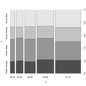
A simple spine plot from a categorical matrix
You can tinker with the graphical parameters to make the chart look “nicer”:
# Custom colours, bar space, and axis labels
spineplot(VADeaths, col = terrain.colors(4),
          off = 5,
          xlab = "Age Class",
          ylab = "Category")
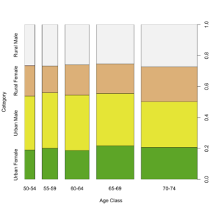
Graphical parameters used to prettify a spine plot
It is hard to resize name labels, as cex, las and so on do not work! The solution is to set these parameters globally using par() and reset them after drawing your plot.
In the following example custom names are also used to help “fit” labels in the plot:
opar <- par(cex.axis = 0.6, las = 2)
spineplot(USPersonalExpenditure,
          xlab = "", ylab = "",
          xaxlabels = c("FT", "HO", "MH", "PC", "PE"))
par(opar)
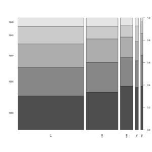
Axis labels are set using par() before drawing a spineplot
The spineplot() function can only deal with 2-dimensional objects. If you have a multi-dimensional table you need to collapse the table to 2D.
spineplot(HairEyeColor)
Error in spineplot.default(HairEyeColor) :
  a 2-way table has to be specified
x <- margin.table(HairEyeColor, margin = c(1,2))
x
       Eye
Hair    Brown Blue Hazel Green
  Black    68   20    15     5
  Brown   119   84    54    29
  Red      26   17    14    14
  Blond     7   94    10    16
spineplot(x, col = c("brown", "blue", "tan", "green"))
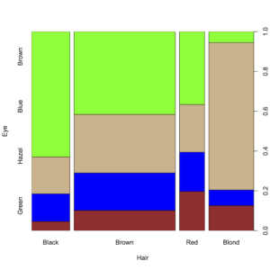
A multi-dimensional table needs to be collapsed to 2D for plotting
A spinogram is a spineplot where the data is in the form factor ~ numeric. A spinogram is analogous to a histogram.
spineplot(tension ~ breaks, data = warpbreaks)
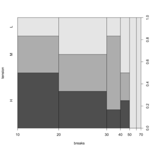
A spinogram is a form of histogram
If you have numeric data you can use factor() to convert the data:
# Use factor(x) to "convert" numeric
spineplot(factor(Month) ~ Ozone,
          data = airquality,
          col = heat.colors(5))
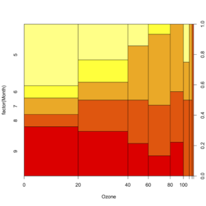
A spinogram where numeric data are converted to a factor before plotting
caption: : A spinogram where numeric data are converted to a factor before plotting
Use the breaks argument as you would for hist() to change the breakpoints (you can enter a single integer or a numeric vector).
spineplot(feed ~ weight, data = chickwts, breaks = 4)
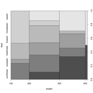
Using the breaks argument to alter the breakpoints in a spinogram
It can be tricky to read a spinogram and it is not trivial to add a legend for the colors. See Tips and Tricks article about legends here.
This article is partly in support of my book An Introduction to R see the publications page for more information.

Drawing mathematical curves using R is fairly easy. Here’s how to plot mathematical functions using R functions curve and plot.
The main functions are curve() and plot.function() but you can simply use plot().
curve(expr, from = NULL, to = NULL, n = 101, add = FALSE,
     type = "l", xname = "x", xlab = xname, ylab = NULL,
     log = NULL, xlim = NULL, ...)

plot(x, y = 0, to = 1, from = y, xlim = NULL, ylab = NULL, ...)
Essentially you use (or make) a function that takes values of x and returns a single value. The arguments are largely self-explanatory but:
expr, x — an expression or function that returns a single result.from, to — the limits of the input (default 0–1).n — the number of “points” to draw (these will be evenly spaced between from and to).... — regular graphical arguments can be used.You can visualize built-in functions. Note that you can use regular graphics arguments to augment the basic plot.
Here is a plot of the sqrt function:
curve(sqrt, from = 0, to = 100, ylab = "Square Root", las = 1)
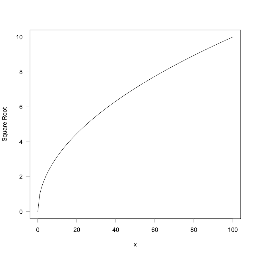
Plot of the square root function sqrt()
Here is a simple log plot:
curve(log, from = 0, to = 100, las = 1, lwd = 2, col = "blue")

Plot of log function using curve()
Use the add = TRUE argument to add a curve() to an existing plot.
curve(sin, -pi*2, pi*2, lty = 2, lwd = 1.5, col = "blue",
      ylab = "Function", ylim = c(-1,1.5))

curve(cos, -pi*2, pi*2, lty = 3, col = "red", lwd = 2, add = TRUE)

# Add legend and title
legend(x = "topright", legend = c("Sine", "Cosine"),
      lty = c(2, 3), lwd = c(1.5, 2),
      col = c("blue", "red"), bty = "n")

title(main = "Sine and Cosine functions")
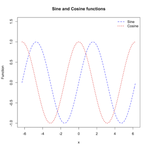
Plot of functions sin and cos using curve()
You can define your own function to plot. Remember that the result should be a single value. In this example we define two functions to convert between Celsius and Fahrenheit:
# Conversion of temperature
cels <- function(x) (x-32) * 5/9
fahr <- function(x) x*9/5 + 32
Now you can use from and to arguments to set the limits for the input (the default is 0–1).
curve(cels, from = 32, to = 100, xname = "Farenheit",
      ylab = "Celsius", las = 1)

curve(fahr, from = 0, to = 50, xname = "Celsius",
      ylab = "Fahrenheit", las = 1)
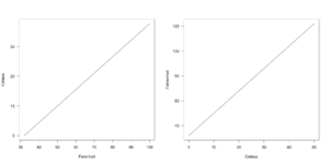
Plots using custom function, temperature conversion
If your function requires additional arguments you need to do something different. In this example you can see the Manning equation, which is used to estimate speed of fluids in pipes/tubes:
manning <- function(r, g, c = 0.1) (r^(2/3) * g^0.5/c)

curve(manning) # fails
Error in manning(x) : argument "g" is missing, with no default
The plotting fails. You need to pre-define all arguments as you cannot “pass-through” additional arguments to your function:
manning <- function(r, g = 0.01, c = 0.1) (r^(2/3) * g^0.5/c)

curve(manning) # works
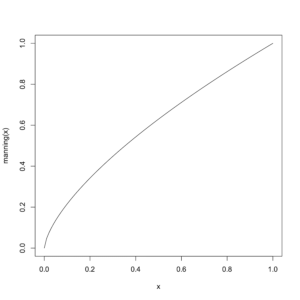
Plot of a custom function with parameters
In the following example you see a built-in function pt() used to visualize the Student’s t distribution.
# pt needs df and lower.tail arguments
PT <- function(x) pt(q = x, df = 100, lower.tail = FALSE)

curve(PT, from = -3, to = 3, las = 1, xname = "t-value",
     n = 20, type = "o", pch = 16, ylab = "probability")
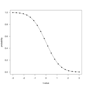
Plot of Student’s t distribution using a function “wrapper”
The workaround is to create a “wrapper” function that calls the actual function you want with the appropriate arguments. Note that in this example the n argument was used to plot 20 points, along with type and pch to create a line with over-plotted points.
This post is part of the support for the new book An Introduction to R. See Publications home page for more details.
Since more people are working from home, from March 2020 all our Data Analytics Training Courses are available as online “conference” events. We’ll be using the Zoom Web Conferencing system. Zoom is easy to use and only requires a small download.
Because of the COVID-19 pandemic and the switch to more home-working we’ve decided to make all our training courses online. The Zoom Web Conferencing system is our choice for delivery. The Zoom software is easy to use and provides a great environment for online learning.
We can run one-to-one training or group events. Zoom is easy to setup and use, it works on all computer operating systems.
Visit our Training Courses page for details about Data Analytics Training Courses.

The formula() is an integral part of the R language. You use a formula to specify relationships between variables for tasks such as graphics and analysis (e.g. linear modelling). Manipulating an R formula is a useful skill.
When you’ve created some kind of analysis model in R you will have specified the variables in some kind of formula. R “recognises” formula objects, which have their own class "formula". If, for example you used the lm() command to create a regression result you will be able to extract the formula from the result.
mod <- lm(Fertility ~ ., data = swiss)
formula(mod)
Fertility ~ Agriculture + Examination + Education + Catholic + Infant.Mortality
It can be useful to be able to extract the components of the model formula. For example you may want to examine how the R2 value alters as you add variables to the model.
To access the parts of a formula you need the terms() command:
terms(formula(mod))
The result contains various components; you want the term.labels.
attr(terms(formula(mod)), which = "term.labels")
[1] "Agriculture" "Examination" "Education" "Catholic"
[5] "Infant.Mortality"
You now have the variables, that is the predictor variables, from the formula. The next step is to get the response variable.
The response variable can be seen using the terms() command and the variables component, like so:
attr(terms(formula(mod)), which = "variables")
list(Fertility, Agriculture, Examination, Education, Catholic, Infant.Mortality)
The result looks slightly odd but essentially it is a list and the 2nd component is the response.
vv <- attr(terms(formula(mod)), which = "variables")
rr <- as.character(vv[[2]]) # The response variable name
rr
[1] "Fertility"
Now you have the response variable, and the predictors from earlier, which you can use to “build” a formula.
In its most basic sense a formula is simply a character string that “conforms” to the formula syntax: y ~ x + z for example. You can build a formula with the paste() command by joining the response, a ~ character and the predictors you want (these themselves separated by + characters).
The following example uses the swiss dataset, which is built into base R.
mod <- lm(Fertility ~ ., data = swiss)

# Get the (predictor) variables
vars <- attr(terms(formula(mod)), which = "term.labels")

# Get the response
vv <- attr(terms(formula(mod)), which = "variables")
rr <- as.character(vv[[2]]) # The response variable name

# Now the predictors
pp <- paste(vars, collapse = " + ")       # All
pp <- paste(vars[1], collapse = " + ")    # 1st
pp <- paste(vars[1:3], collapse = " + ")  # 1,2,3

# Build a formula
fml <- paste(rr, " ~ ", pp)
fml
[1] "Fertility ~ Agriculture + Examination + Education + Catholic + Infant.Mortality"
Once you have your formula as a character object you can use it in place of a regular formula in commands.
The character string representing a formula can be used exactly as you would a “regular” formula:
lm(fml, data = swiss)
Call:
lm(formula = fml, data = swiss)

Coefficients:
     (Intercept)       Agriculture       Examination         Education
         66.9152           -0.1721           -0.2580           -0.8709
        Catholic  Infant.Mortality
          0.1041            1.0770
One use for building a formula is in model testing. For example you create your regression model containing five predictors but maybe only the first three are really necessary. You can re-build the formula term by term and extract the R2 value for example. This would show you how the explained variance alters as you add more variables.
See more articles in our Tips and Tricks pages.

A histogram is a standard way to present the distribution of a sample of numbers. A basic histogram is useful but it is easy to add more to a histogram in R to produce an even more informative plot. In this article you’ll see how to add a rug and a strip-chart to a basic historgram using simple R commands.
It is easy to make a histogram using R with the hist() command. For example:
set.seed(123)
x <- norm(n = 50, mean = 10, sd = 1)
hist(x, col = "skyblue")
Produces a histogram resembling this:

A rug plot can be added to more or less any graphic. The rug() command can add the rug to any side of the plot:
side = 1 is the bottom axisside = 2 is the left axisYou can alter the colour and width of the rug lines using regular graphical parameters:
rug(x, side = 1, col = "blue")
Adds the rug like so:

A strip chart can also be added to any chart via the stripchart() command. However, you also need to specify add = TRUE to the command. Giving a bit of jitter helps to separate out points that are coincident:
stripchart(x,
           method = "jitter",
           pch = 23,
           bg = "pink",
           add = TRUE)
The final plot looks like so:

There are many additional options for the stripchart() command; use help(stripchart) in R to find out more. Look out for other articles in our Tips & Tricks pages.
Sometimes you know you are in for a bit of a wait when you’re running some R code. However, it would be nice to get some idea of how long you’ll be waiting. A progress indicator for the R console is what you need.
The txtProgressBar() command can help you here. The command allows you to set-up a progress indicator that displays in the R console and shows your progress towards the “end point”.
txtProgressBar(min, max, style)
You set the starting and ending points via the min and max parameters, usually these will match up with the “counter” in a loop. The style parameter is a simple value, style = 3 shows a series of = characters marching towards the % completion (displayed at the end of a line in your console).
The setTxtProgressBar() command actually updates the progress indicator and displays in the console. When you are done you close()the progress bar to tidy up.
pb <- txtProgressBar(min = 0, max = 100, style = 3)
  for(i in 1:100) {
    Sys.sleep(0.1)
    setTxtProgressBar(pb, i)
    }
close(pb)
The first line sets up the progress indicator. The for() command sets a loop to run from 0 to 100. The loop in this example is trivial with the Sys.sleep() command simply making R “wait” 0.1 seconds; in your own code you would replace this line with your own routines. The 4th line updates the progress indicator. After the loop has ended the close() command “resets” the progress bar.