Logistic regression: model prediction
Exercise 11.3.1.
Statistics for Ecologists (Edition 2) Exercise 11.3.1
These notes are about how to use the results of a regression model to predict the value of the response variable when you supply certain values of the predictor.
Predicting values from logistic regression and other models
Introduction
When you carry out a regression you are looking to describe the data in terms of the variables that form the relationships. When you’ve got your regression model you are able to describe the relationship using a mathematical model (which is what the regression model is).
You can use the regression model to make predicted values, which is where you use “new” values of the predictor (that is ones not observed in the original dataset) to predict the response variable.
These predicted values are especially important in logistic regression, where your response is binary, that is it only has two possibilities. The result you get when you “predict” response values in a logistic regression is a probability; the likelihood of getting a “positive” result when the predictor variable is set to a particular value.
These notes will show you how to use the predict() command in R to produce predicted values for regression models, particularly logistic regression.
The predict() command
The predict() command is used to compute predicted values from a regression model. The general form of the command is:
predict(model, newdata, type) |
|
| model | A regression model, usually the result of lm() or glm(). |
| newdata | A data.frame giving the values of the predictor(s) to use in the prediction of the response variable. |
| type | The type of prediction, usually you want type = “response”. |
The model is simply the result of a regression model. You need to specify type = “response” so that your prediction predicts the response variable (note that this is not necessarily the default, so you must specify it).
The newdata parameter is where you specify the values of the predictor(s) that you want to use to predict the response variable. You can make a data.frame object containing the variables (with variable names to match the original dataset), or can specify it “on the fly”. You’ll see examples shortly.
Prediction in logistic regression
Logistic regression is carried out in cases where your response variable can take one of only two forms (i.e. it is binary). There are two general forms your response variable can take:
- Presence/absence, that is, 0 or 1 (or some other binary form).
- A success/failure matrix, where you have two frequencies for each observation (the “successes” and the “failures”).
The way your data are arranged does not make much difference to how you carry out the predictions but because of the different forms it is useful to see an example of each.
Logisitc regression and presence/absence
When you have the response variable as presence/absence (1 or 0) it is easy to see that your response is in binary form. The logistic regression converts the 1s and 0s to a likelihood (under the various levels of your predictor variables), so your result is in that form. So, when you use the predict() command you can get the probability of getting a success (a presence: 1).
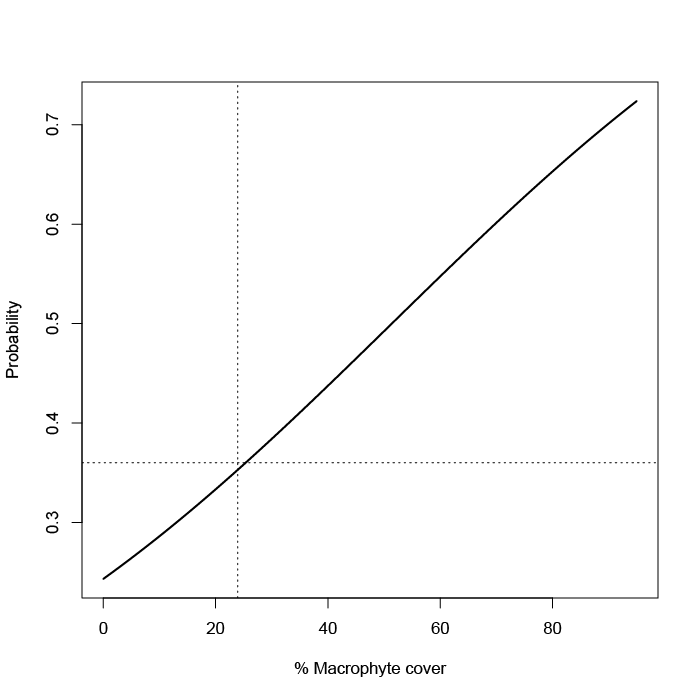
The example file (Predict regressions.RData) contains a dataset that looks at the presence or absence of an amphibian (great crested newt) in ponds. The data are called gcn. Various habitat factors were measured. One factor is the percentage cover of macrophytes. You can use the logistic regression to explore the relationship between the presence (or absence) of newts and the cover of macrophytes.
Once you have the regression model you can use predict() to predict the likelihood of finding a newt given any value for the cover of macrophytes.
Make a regression model
Make a regression model result:
gcn.glm <- glm(presence ~ macro, data = gcn, family = binomial)
The result is that the macro variable is statistically significant:
Coefficients:
             Estimate Std. Error z value Pr(>|z|)
(Intercept) -1.135512   0.217387  -5.223 1.76e-07 ***
macro        0.022095   0.005901   3.744 0.000181 ***
You can present a graph of the model (see the book text for the code):

Predict outcomes
Now you could look at the line on the plot (made using fitted values) and estimate the probability of finding a newt (presence = 1) for any percentage cover of macrophyte. Alternatively you can use the predict() command.
nd = data.frame(macro = c(40, 50, 60))
nd
  macro
1    40
2    50
3    60

predict(gcn.glm, newdata = nd, type = “response”)
        1         2         3
0.4374069 0.4923162 0.5474114
See that you first make a data.frame with a variable called macro, to match the original data. This new data is used to predict the response. However, the value you get is not exactly a response but it is the likelihood of “success”, that is finding a newt. You could have set the original response variable (presence) to have been 1 for absence and 0 for presence. Apart from being a little odd you’d be assuming that a “success” was the absence of the newts.
In any event your prediction is a probability of success. You might have chosen to create the prediction newdata data.frame directly in the predict() command, which is what you’ll see in the following example.
Logistic regression and success/failure matrix
Your data may be in a subtly different form to the 0 or 1 model. In the following example you have a predictor variable, latitude, and a response but the response is split into two frequencies:
cbh
  latitude Mpi90 Mpi100  p.Mpi100
1     48.1    47    139 0.7473118
2     45.2   177    241 0.5765550
3     44.0  1087   1183 0.5211454
4     43.7   187    175 0.4834254
5     43.5   397    671 0.6282772
6     37.8    40     14 0.2592593
7     36.6    39     17 0.3035714
8     34.3    30      0 0.0000000
Here you have two versions of an allele in the Californian beach hopper. The data are in the file (Predict regressions.RData) and are called cbh. For each sampling latitude a number of animals were collected. They can have one form of the allele or the other. So your response variable is split into the frequency of each. If you take those two variables you have a success/failure matrix.
The logistic regression can constrict the likelihood from the success/failure. It does not matter which allele you choose to be the “success” but here I’ve used the Mpi100 allele (because the proportion increases with latitude). The proportion of the “success” is shown in the final column. It won’t be used in the regression except to draw a plot.
Make a regression model

Start by making a regression model. You need to make a success/failure matrix but this can be done as part of the glm() command formula.
cbh.glm <- glm(cbind(cbh$Mpi100, cbh$Mpi90) ~ latitude, data = cbh, family = binomial)
The result shows that latitude is a significant variable:
Coefficients:
            Estimate Std. Error z value Pr(>|z|)
(Intercept) -7.64686    0.92487  -8.268   <2e-16 ***
latitude     0.17864    0.02104   8.490   <2e-16 ***
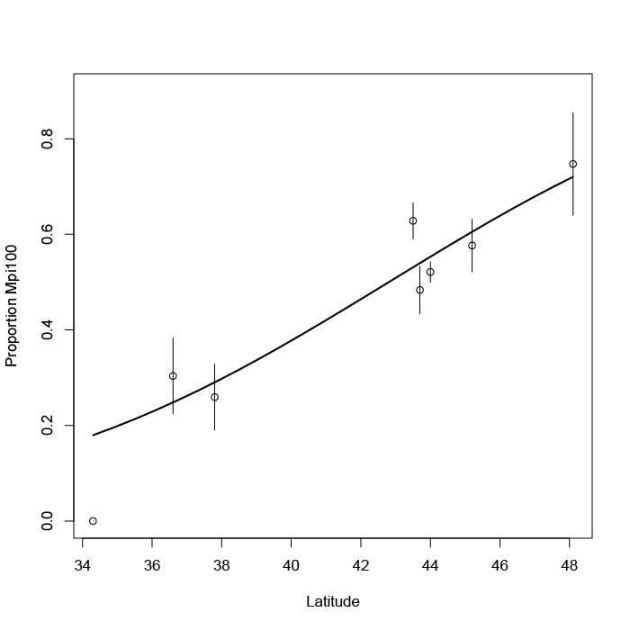
You can draw this as a plot (because of the replicates we can add error bars):
Predict outcomes
As before you could use the plot to predict the likelihood of “success”, the Mpi100 allele. You can also use the predict() command:
predict(cbh.glm, newdata = data.frame(latitude = c(35, 40, 45)), type = "response")
        1         2         3
0.1986945 0.3772411 0.5967457
Note that this time the newdata parameter used a data.frame created on the fly.
Prediction with multiple predictors
When you have multiple predictor variables you have to specify them all in the newdata parameter of the predict() command. It is easiest to make a new data.frame object to hold these “new” data unless you only have one or two values.
In the following data example there are four predictors and one response (Length).
names(mf)
[1] "Length" "Speed"  "Algae"  "NO3"    "BOD"
The data give the lengths of a freshwater invertebrate (a mayfly species) and some habitat conditions at the sampling locations where each observation took place. The data are in the file (Predict regressions.RData) and are called mf.
Your new data.frame has to have the same variable names but they do not have to be in any order. You only have to include variables that are in the regression model.
Make the regression model
Make the model:
mf.lm <- lm(Length ~ BOD + Algae, data = mf)
The result shows the coefficients (one variable is not significant but we’ll leave it in).
Coefficients:
            Estimate Std. Error t value Pr(>|t|)
(Intercept) 22.34681    4.09862   5.452 1.78e-05 ***
BOD         -0.03779    0.01517  -2.492   0.0207 *
Algae        0.04809    0.03504   1.373   0.1837
Predict the result
Because there are two predictors it is not practical to draw a plot (apart from diagnostics, see Exercise 11.1). So the predict() command is the way to go.
predict(mf.lm, newdata = data.frame(BOD = 20, Algae = 10), type = “response”)
       1
22.07199
You can of course make a separate data.frame containing BOD and Algae columns and populate it with values for which you want to get a prediction.
Data examples
The data examples used here are available as part of the support data for the book. I’ve also added a file Predict regressions.RData, which contains just the three datasets mentioned on this page.
Comments are closed.