Association Plots
Association plots in R. An association plot draws the results of an association test by charting the Pearson Residuals.
Association plots in R are drawn using assocplot()
assocplot(x, col = c("black", "red"), space = 0.3,
          main = NULL, xlab = NULL, ylab = NULL)
| Parameter | Explanation |
|---|---|
x |
the data, usually a numeric matrix. |
col |
colors for positive and negative associations. |
space |
amount of space between the bars, as a fraction of average bar height and width (default = 0.3). |
main, xlab, ylab |
title annotations. |
Essentially you need a 2-dimensional matrix to use assocplot():
VADeaths
      Rural Male Rural Female Urban Male Urban Female
50-54       11.7          8.7       15.4          8.4
55-59       18.1         11.7       24.3         13.6
60-64       26.9         20.3       37.0         19.3
65-69       41.0         30.9       54.6         35.1
70-74       66.0         54.3       71.1         50.0
Apart from the titles, the only graphical parameter you can alter directly is col, to alter the positive and negative bar colors:
assocplot(VADeaths, col = c("lightblue", "pink"),
	  xlab = "Age class", ylab = "Driver actegory")

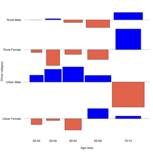
Basic association plot using custom color for positive and negative bars
Graphical parameters
If you want to alter the general appearance of your association plot you’ll need to set the appropriate graphical parameters using par() before using assocplot():
opar <- par(las = 1, cex = 0.8, mar = c(5,7,2,1))

assocplot(VADeaths, col = c("blue", "tomato"),
          space = 0.05, xlab = "Age class")
title(ylab = "Driver category", line = 6)

par(opar)

Custom graphical parameters have to be applied using par() before using assocplot()
In the preceding example the margins were widened to allow the labels to “fit”. Note also how title() was used to place the y-axis annotation on an outer line.
Data layout
Essentially you need a 2D matrix for assocplot() to make an association plot in R. If you have something else you need to coerce it to the correct form.
Here are some options:
data.frameuseas.matrix()to alter the form.tableusex[r, c, n, ...]to “pick out” the appropriate 2D sub-table or..tableusemargin.tableto “collapse” a table and combine across the margins you want.
# 3D table
HairEyeColor
, , Sex = Male

       Eye
Hair    Brown Blue Hazel Green
  Black    32   11    10     3
  Brown    53   50    25    15
  Red      10   10     7     7
  Blond     3   30     5     8

, , Sex = Female

       Eye
Hair    Brown Blue Hazel Green
  Black    36    9     5     2
  Brown    66   34    29    14
  Red      16    7     7     7
  Blond     4   64     5     8
# Choose "Male"
HairEyeColor[,,1]
       Eye
Hair    Brown Blue Hazel Green
  Black    32   11    10     3
  Brown    53   50    25    15
  Red      10   10     7     7
  Blond     3   30     5     8
# Combine "Male" and "Female"
margin.table(HairEyeColor, margin = c(1,2))
       Eye
Hair    Brown Blue Hazel Green
  Black    68   20    15     5
  Brown   119   84    54    29
  Red      26   17    14    14
  Blond     7   94    10    16
# Combine "Eye"
margin.table(HairEyeColor, margin = c(1,3))
       Sex
Hair    Male Female
  Black   56     52
  Brown  143    143
  Red     34     37
  Blond   46     81
Alternatives to assocplot()
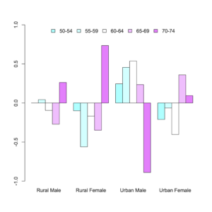
The assocplot() function is not the only was to draw an association plot using R. You could run a chisq.test() and extract the Pearson residuals $residuals, which you then plot using barplot().
X <- chisq.test(VADeaths)
X$residuals
         Rural Male Rural Female Urban Male Urban Female
50-54 -0.0001229145  -0.09956533  0.2454344  -0.21106734
55-59  0.0422284686  -0.56107962  0.4550546  -0.06391943
60-64 -0.0951496863  -0.16808112  0.5368919  -0.40335827
65-69 -0.2718462679  -0.34870589  0.2349807   0.36003546
70-74  0.2624133483   0.73510055 -0.8898149   0.09370444
barplot(X$residuals, beside = TRUE, col = cm.colors(5),
        ylim = c(-1,1), legend = TRUE,
	args.legend = list(x = "top", bty = "n", ncol = 5))
title(ylab = "Pearson residuals", xlab = "Category")

Alternative to assocplot() is to use barplot() on the Pearson residuals
To get multiple rows, with a separate mini-plot for each row you would need to set-up par(mfrow = c(rows, cols)).
There are potential advantages to this method, for example you can add horizontal lines at +/- 2 to show the “significance band”. However, it is also somewhat more involved!
This article is partly in support of my book An Introduction to R see the publications page for more information.
- An Introduction to R will be published by Pelagic Publishing. See all my books at Pelagic Publishing.
- For more articles look at the Tips and Tricks page and look for the various categories or use the search box.
- See also the Knowledge Base where there are other topics related to R and data science.
- Visit our other site at GardenersOwn for a more ecological matters.
