Types of R object – 1. basics

R “recognises” various sorts of object. Every object holds a class attribute, which controls how the object is dealt with by various commands.

At the most basic level you can think of R objects as being in one of three main forms:

  • numeric
  • character
  • factor

Object type: basics

The numeric type is obvious – numbers:

> num <- c(2.3, 4.1, 5, 12.2)
> num
[1] 2.3 4.1 5.0 12.2

> class(num)
[1] "numeric"

The character type is also obvious – text:

> chr <- c("a", "b", "c")
> chr
[1] "a" "b" "c"

> class(chr)
[1] "character"

The last basic type is a factor. The factor can appear like a number or a character, depending upon its contents:

> fact <- gl(3, 2)
> fact
[1] 1 1 2 2 3 3
Levels: 1 2 3

> class(fact)
[1] "factor"

The previous object (fact) looks like numbers. The following looks superficially like characters:

> fac <- gl(3, 2, labels = c("p", "q", "r"))
> fac
[1] p p q q r r
Levels: p q r

> class(fac)
[1] "factor"

In fact, you can see that it is not a character object because the text items do not have quotes around them. Another “clue” is the Levels: part of the display – but beware because this is not always displayed.

Factor objects are important and are used in many statistical analyses. When you import data using read.csv() for example, the columns of text are converted to factor objects unless you explicitly tell R otherwise.

Be classy: object class attributes in R

All R objects have a class attribute. This can be viewed (or set) via the class() command. The class can be any character string and an object can hold more than one class. You can use the class to help you identify what sort an object is, for example:

> bird
               Garden Hedgerow Parkland Pasture Woodland
Blackbird          47       10       40       2        2
Chaffinch          19        3        5       0        2
Great Tit          50        0       10       7        0
House Sparrow      46       16        8       4        0
Robin               9        3        0       0        2
Song Thrush         4        0        6       0        0

At first glance you cannot tell if this object is a data.frame or a matrix. The class() command can help you find out:

> class(bird)
[1] "matrix"

Some commands can be pressed into service for special classes – for example plot(), summary() and print() commands can be written to process objects of a specific class. You simply name your custom command to append the class; for example plot.lm(), print.lm() or summary.lm() commands, which are part of the basic distribution of R. When you issue a plot() command for example R looks at the class of the object to see if there is a plot.xxxx() command to match (where xxxx is the class of the object). If there is then this custom command is carried out. If a custom command is not available then the basic plot() command is used.

The class attribute is often used in functions to check that an object is of the right sort before carrying out the commands.

Add comments to objects in R

All R objects have attributes – one of these can be a comment. You can set or view the comment attribute of an object using the comment() command. For example:

> x <- c(2, 3, 5, 4, 3, 6)
> comment(x)
NULL

> comment(x) <- "A simple numeric variable"
> comment(x)
[1] "A simple numeric variable"

You have more than one comment, use the square brackets to “define” additional comments.

> comment(x)[2] <- "A second note"
> comment(x)
[1] "A simple numeric variable" "A second note"

Use the comment to remind you what the object is – it is easy to forget later.

NA items in R data

The NA item is a special object and represents “Not Available”. Sometimes this is because data were genuinely not collected but often it is because you have unequal columns and your data frame is padded out with NA to make the short columns longer. The na.rm = TRUE instruction can be used to strip out NA items before some commands, for example:

> x
[1] 2 4 3 6 2 8 NA NA

> mean(x)
[1] NA

> mean(x, na.rm = TRUE)
[1] 4.166667

However, this does not always work:

> length(x, na.rm = TRUE)
Error in length(x, na.rm = TRUE) :
2 arguments passed to ‘length’ which requires 1

In this case the na.omit() command can be used to strip out the NA items:

> length(na.omit(x))
[1] 6

Interactive file choice in R

You can use the file.choose() command instead of the filename when reading a file. This works for Windows or Mac operating systems (in Linux you need to type the “filename” in full). Use file.choose() instead of the filename for reading data with read.csv() or for getting scripts with the source() command for example. You can also use it to write files as long as the file already exists, for example for saving the workspace via the save.image() command.

Keyboard shortcuts in Excel

If you have a lot of rows and/or columns in your spreadsheet it can be a real pain navigating from one spot to another. Selecting many rows of data is also a tedious operation. The trick is to learn some of the keyboard shortcuts, key-combinations that can save you a lot of time and effort. Note that these only work for Windows versions of Excel.

Named ranges

All cells have a row and column reference, which is shown in a box (the Name Box) to the left of the formula bar. You can type a cell reference in this box to jump directly to a cell. This works fine if you know the column and row number of the cell you want – of course A1 will always take you to the top of your worksheet.

If you select one or more cells and type a name in the Name Box you assign a name to those cells (the cells do not have to be adjacent to one another). Later, you can type the name to jump to the location defined by the name. You can also use the drop-down icon and select a name. If your name “points” to several cells they are all selected.

The Name Box is not quite a keyboard shortcut, but it links the Named Ranges to the keyboard shortcuts you’ll see next.

Moving around and selecting with arrow keys

There are two important “key modifiers” that you need in conjunction with the arrow keys:

  • Ctrl
  • Shift

The control (Ctrl) key allows you to jump rapidly from one end of a block to another. The Shift key allows you to select cells.

If you hold the Ctrl key and press the arrows you’ll jump in the direction of the arrow. The distance of the jump depends on the data, if there are data in the row or column you’ll go to the end of the current block of data. If you press Ctrl+Arrow again you’ll jump to the start of the next block, press Ctrl+Arrow again and you’ll jump to the end of that block. If there are no data you’ll travel to the extreme edge of the worksheet, which can be hundreds or thousands of rows/columns, depending on your version of Excel.

The Shift key allows you to select cells. If you click in a cell, then press Shift+Arrow you’ll select cells in the direction of the arrow.

Using Ctrl+Shift+Arrow allows you to select a block of data in a row or column. Thus you can highlight many rows and/or columns of data quickly and easily.

Selecting “everything”

You can select everything using the space between the row and column headers, which contains a triangle. Clicking in the box selects the entire worksheet, including empty cells. This is not always what you want so you can use Ctrl+A to select all the data.

However, Ctrl+A does not work how you might expect. If you click in a block of data then press Ctrl+A the block of data will be selected, if there are other data cells they will not be selected if there are empty cells between the blocks. The selection is rectangular so if one row or column is bigger than the others, the selection area is expanded to incorporate the cells.

If you click a cell adjacent to a block of data and type Ctrl+A the block of cells next to the insertion point will become selected. You can position the insertion point so that several blocks of data become selected, essentially Excel looks at the cells surrounding the insertion point and expands the selection to include any non-empty cells. This is how you can get a chart or a Pivot Table without having to select any data. Knowing this behaviour also allows you to insert blank charts, by ensuring that the insertion point is not in, or adjacent to, any data.

Selecting using the mouse

The Ctrl and Shift keys can be used with the mouse. The Ctrl key allows you to select non-adjacent cells or cells in a non-rectangular block. The Shift key “fills in” the selection between the first block you select and subsequent blocks. This behaviour extends to entire rows or columns, so you can click in the headers to select several rows or columns.

Selecting data from menus

The shortcuts can be used in conjunction with various menu windows. For example, if you are selecting data for a chart using the Select Data button. You can click the topmost cell in a column for example and extend down the entire block using Ctrl+Shift+Down Arrow. This is helpful when you have many rows of data.

Named Ranges in Excel

When you’ve got a lot of rows of data in your worksheet it can be quite tedious to use the mouse to highlight or select them every time you want to use a formula or make a chart. Using named ranges can take some of the tedium out of this process (keyboard shortcuts can also help but I’ll deal with them another time).

You can make any selection into a named range. There are two main ways:

  • Select some cells and type the name into the Name Box.
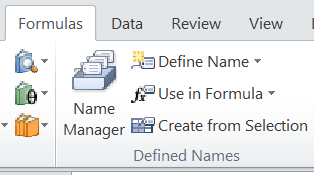
  • Use the Defined Names section of the Formulas

The Name Box usually shows you the row and column reference of the currently active cell, you can type a cell reference into the box to jump directly to that location.

To define a named range, you can select some cells then type a name into the Name Box. Excel doesn’t like spaces, which will convert to underscore. The trick is to keep names short, but meaningful. Any defined names will appear when you click the triangle icon in the Name Box.

If you click a name, you’ll select the cells linked to that named range. You’ll probably have your data arranged so that each column is a separate variable. The easy way to define names for all the columns is to use the Formulas > Create from Selection button.

First select all the data, click once anywhere in the data then hit Ctrl+A on the keyboard. Then go to the Formulasmenu and click the Create from Selection button. You can now decide where the names are, usually they’ll be the top row but there are other options.

Now the names are defined you’ll see the names in the Name Box. The names can be used any time you need a cell range and are not case sensitive. In fact, if you start to type a name in a formula you’ll see any matching named ranges appear in a pop-up (along with function names).

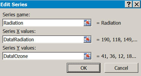
You can also use names in defining charts but you’ll generally have to give the worksheet name too, e.g. Data!Ozone selects the named range Ozone from the Dataworksheet.

The Formulas > Name Manager button allows you to manage the named ranges, you can edit or delete items.

Roman Numerals in Excel

You can convert between Roman numerals and regular Arabic numbers using the ROMAN and ARABIC functions.

Regular (Arabic) numbers to Roman numerals

The ROMAN function takes a regular number and gives you the Roman equivalent. There is an additional parameter you can add, to control the appearance of the final Roman number:

=ROMAN(number, form)

The number is simply the number you want to convert (usually you’ll give the cell reference). You specify the form as a value from 0–4 or as a logical (TRUE or FALSE) like so:

  • In general, the larger the number you use for form the more concise the final Roman numeral becomes.
  • If you use 0 or don’t put any value for form you get the classic form.
  • If you specify TRUE you get the classic form.
  • If you specify FALSE you get the most consice form.

The Excel help entry for this function shows an example for 499 to illustrate the effect of altering the form parameter.


=Roman(499, form) Result
0, TRUE or omitted CDXCIX
1 LDVLIV
2 XDIX
3 XDIX
4 or FALSE ID

Roman numerals to regular (Arabic) numbers

Since Excel version 2013 you can convert a number in Roman form to a regular Arabic number; you use the ARABIC function. There is only one parameter, the number you wish to convert (usually you’ll give this as a cell reference). It does not matter what form the number is in (see above), it will be evaluated. The function is not case sensitive.

You can specify your number in any number of ways, not strictly in Roman form. As long as you use “allowable” Roman characters the ARABIC function will evaluate the result e.g.

=ARABIC(XXICD) produces 379 but the reverse, =ROMAN(379) is CCCLXXIX regardless of how concise you are.

The ARABIC function is available in Excel 2013 and Open Office 4.x (and Libre Office) but not in older versions.

Reversing the axis of an Excel chart

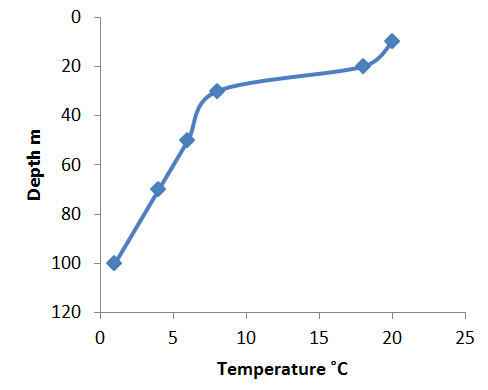
Sometimes you want to make a plot that reflects the “real” situation rather than a plain “mathematical” one. An example might be temperature and depth of the ocean. You ought to plot the temperature on the y-axis and the depth on the x-axis but it would be nice to visualize the change in temperature with depth as if you were looking down a profile of the ocean. Your first attempt makes a scatter plot but the vertical is upside down with the deeper values at the top.

I am text block. Click edit button to change this text. Lorem ipsum dolor sit amet, consectetur adipiscing elit. Ut elit tellus, luctus nec ullamcorper mattis, pulvinar dapibus leo.

If you select the box that says Values in reverse order the values will… reverse. The x-axis will still be at the top so you might want to alter it using the Horizontal axis crosses: section. Set the x-axis to cross at the Maximum axis valueand it will move to the bottom (the values are in reverse order now so the max. value is at the bottom of the y-axis).

Now your chart is the way up you intended. Here I added smoothed joining lines to help visualize the pattern of temperature with depth. Right-click on a data point and select Format Data Series… to bring up the options.

Adding data series to an Excel chart

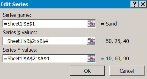
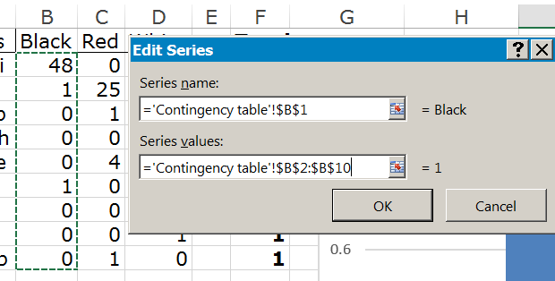
So, you’ve used the Insert menu item to select a chart type and need to add some data. Make sure that you click once on the blank chart and select the Home > Chart Tools > Design menu. Click the Select Data button and you will see a menu window that will allow you to “build” a chart. If your graph is blank, you’ll be able to select data and if your graph already contains data you’ll be able to add extra data series and edit/modify existing data.

Use the Add button on the left to choose the data. You’ll be able to select:

  • A name for the series (this will appear in any legend).
  • The values for the y-axis.
  • Values for the x-axis.

If your data are a scatter plot with x,y values then the values will appear in the box on the right once you return to the Select Data Source menu. If the data are categorical (or you do not select any), you can select the data using the Edit button on the right side of the Select Data Source menu box.