
Drawing mathematical curves
Drawing mathematical curves using R is fairly easy. Here’s how to plot mathematical functions using R functions curve and plot.
The main functions are curve() and plot.function() but you can simply use plot().
curve(expr, from = NULL, to = NULL, n = 101, add = FALSE,
     type = "l", xname = "x", xlab = xname, ylab = NULL,
     log = NULL, xlim = NULL, ...)

plot(x, y = 0, to = 1, from = y, xlim = NULL, ylab = NULL, ...)
Essentially you use (or make) a function that takes values of x and returns a single value. The arguments are largely self-explanatory but:
expr,x— an expression orfunctionthat returns a single result.from,to— the limits of the input (default0–1).n— the number of “points” to draw (these will be evenly spaced betweenfromandto)....— regular graphical arguments can be used.
Simple Math and Trigonometry
You can visualize built-in functions. Note that you can use regular graphics arguments to augment the basic plot.
Here is a plot of the sqrt function:
curve(sqrt, from = 0, to = 100, ylab = "Square Root", las = 1)
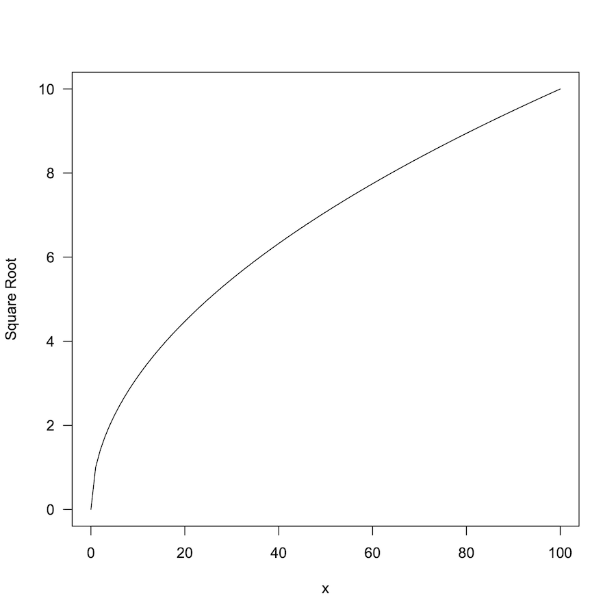
Plot of the square root function sqrt()
Here is a simple log plot:
curve(log, from = 0, to = 100, las = 1, lwd = 2, col = "blue")

Plot of log function using curve()
Adding to plots
Use the add = TRUE argument to add a curve() to an existing plot.
curve(sin, -pi*2, pi*2, lty = 2, lwd = 1.5, col = "blue",
      ylab = "Function", ylim = c(-1,1.5))

curve(cos, -pi*2, pi*2, lty = 3, col = "red", lwd = 2, add = TRUE)

# Add legend and title
legend(x = "topright", legend = c("Sine", "Cosine"),
      lty = c(2, 3), lwd = c(1.5, 2),
      col = c("blue", "red"), bty = "n")

title(main = "Sine and Cosine functions")
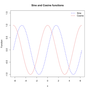
Plot of functions sin and cos using curve()
Custom functions
You can define your own function to plot. Remember that the result should be a single value. In this example we define two functions to convert between Celsius and Fahrenheit:
# Conversion of temperature
cels <- function(x) (x-32) * 5/9
fahr <- function(x) x*9/5 + 32
Now you can use from and to arguments to set the limits for the input (the default is 0–1).
curve(cels, from = 32, to = 100, xname = "Farenheit",
      ylab = "Celsius", las = 1)

curve(fahr, from = 0, to = 50, xname = "Celsius",
      ylab = "Fahrenheit", las = 1)
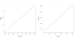
Plots using custom function, temperature conversion
Function arguments
If your function requires additional arguments you need to do something different. In this example you can see the Manning equation, which is used to estimate speed of fluids in pipes/tubes:
manning <- function(r, g, c = 0.1) (r^(2/3) * g^0.5/c)

curve(manning) # fails
Error in manning(x) : argument "g" is missing, with no default
The plotting fails. You need to pre-define all arguments as you cannot “pass-through” additional arguments to your function:
manning <- function(r, g = 0.01, c = 0.1) (r^(2/3) * g^0.5/c)

curve(manning) # works
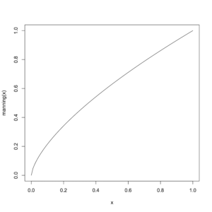
Plot of a custom function with parameters
In the following example you see a built-in function pt() used to visualize the Student’s t distribution.
# pt needs df and lower.tail arguments
PT <- function(x) pt(q = x, df = 100, lower.tail = FALSE)

curve(PT, from = -3, to = 3, las = 1, xname = "t-value",
     n = 20, type = "o", pch = 16, ylab = "probability")
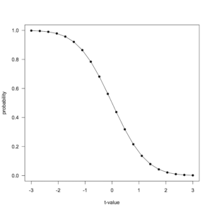
Plot of Student’s t distribution using a function “wrapper”
The workaround is to create a “wrapper” function that calls the actual function you want with the appropriate arguments. Note that in this example the n argument was used to plot 20 points, along with type and pch to create a line with over-plotted points.
This post is part of the support for the new book An Introduction to R. See Publications home page for more details.
- An Introduction to R will be published by Pelagic Publishing. See all my books at Pelagic Publishing.
- For more articles visit the Tips and Tricks page and look for the various categories or use the search box.
- See also the Knowledge Base where there are other topics related to R and data science.
- Look at our other books on the Publications Page.
- Visit our other site at GardenersOwn for a more ecological matters.
Comments are closed.