Legends on graphs and charts
Exercise 6.3.1a.
Statistics for Ecologists (Edition 2) Exercise 6.3.1a
These notes about legends in graphs/charts supplement the text in Chapter 6.
Legends on graphs and charts
Introduction
A legend is a tool to help explain a graph. You are most commonly going to want to add one to a bar chart where you have several data series. You’ll also want to add one to a line or scatter plot when you have more than one series. Essentially you use a legend to help make a complicated plot more understandable.
In R you can add a legend to any plot using the legend() command. You can also use the legend = TRUE parameter in the barplot() command. The barplot() command is the only general plot type that has a legend parameter (the others need a separate legend).
The legend() command has a host of parameters, which can be tweaked to produce the finished article. Generally, the most difficult part is making room on the chart for the legend itself!
Legend Essentials
The legend() command has a wealth of parameters at its disposal. This gives it a great deal of flexibility and customizability <sic> but this also makes it daunting and hard to get to grips with.
The legend() command has the following general form:
legend(x, y = NULL, legend, col, pch, lty, lwd, fill, border, bty, ncol, y.intersp)
| x, y = NULL | The co-ordinates to place the legend (its top-left corner). You can also specify a shortcut location as a text string: “top”, “right”, “bottomleft” and so on, which allows a general spot to be filled quickly. |
| legend | The text to be used for the legen entries. The default is taken from the data. |
| col | The colors to be used for lines or points that appear in the legend. |
| pch | The plotting character(s) to use. |
| lty | The line type (style) to use. |
| lwd | The line width to use. |
| fill = NULL | A set of colors to appear in boxes beside the legend text entries. If NULL (the default) an empty box is placed. To suppress the box omit the fill parameter. |
| border = “black” | The border color for the box if fill is specified (as a color or NULL). |
| bty = “o” | The border type for the overall legend, use bty = “n” for no border. |
| ncol = 1 | The number of columns for the legend, the default is 1 (i.e. a vertical legend). |
| y.intersp = 1 | The width between legend lines, set >1 to space the lines out. There is also a x.intersp parameter, which operates horizontally. |
There are a number of other parameters that I’ve not listed. The ones here are the most essential.
When adding a legend you need to make sure that the items in the legend() command match the parameters you set in the plotting command. It helps to specify pch, col, lty and so on explicitly in the plotting command, as you can match the parameters more easily than if you relied on the defaults.
The barplot() command is the only general plotting command that has a legend parameter. You can pass additional parameters to the legend using the args.legend parameter, as you’ll see shortly.
Adding legends from the barplot() command
The barplot() command allows use of a legend parameter, which calls legend() with its basic settings. You can pass parameters to the legend() command by adding args.legend and giving the details as a list().
The biggest problem is usually how to make appropriate space for the legend to fit in the plot window. There are two main options:
- Alter the axis size to give extra room (vertically or horizontally).
- Place the legend into the plot margin.
The following examples use a matrix dataset that gives the abundance of some butterfly species at a site over several sample years:
> bf
        1996 1997 1998 1999 2000
M.bro     88   47   13   33   86
Or.tip    90   14   36   24   47
Paint.l   50    0    0    0    4
Pea       48  110   85   54   65
Red.ad     6    3    8   10   15
Ring     190   80   96  179  145
> class(bf) # Check you have a matrix
[1] "matrix"
You can get the sample data here: butterfly.RData.
Altering the y-axis to make room
In a basic plot there will often not be enough room to accommodate the legend:
> barplot(bf, legend = TRUE)
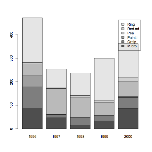
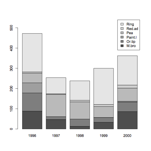
Note that the default location for the legend is “topright”. In this case the simplest way to make room is to resize the y-axis using the ylim parameter.
> barplot(bf, legend = TRUE, ylim = c(0,550))
A simple rescale of the y-axis will often allow the legend to fit.
You may have to play around with the axis setting to get the best values to use.
Pass legend parameters via barplot()
To pass parameters (arguments) to the legend() command from barplot() the parameters need to be passed as a list() with the args.legend parameter.
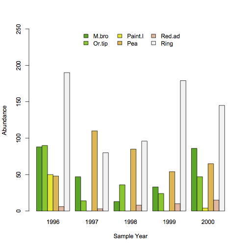
> barplot(bf, beside = TRUE, col = terrain.colors(6), ylim = c(0, 250), legend = TRUE, args.legend = list(bty = “n”, x = “top”, ncol = 3))
title(xlab = “Sample Year”, ylab = “Abundance”)
In this case the y-axis is lengthened and additional parameters passed to legend(). The legend box is suppressed (bty = “n”), placed at the top center (x = “top”), and made into 3 columns (ncol = 3).
Altering the x-axis to make room

You can alter the x-axis using the xlim parameter, which allows you to place the legend at the right.
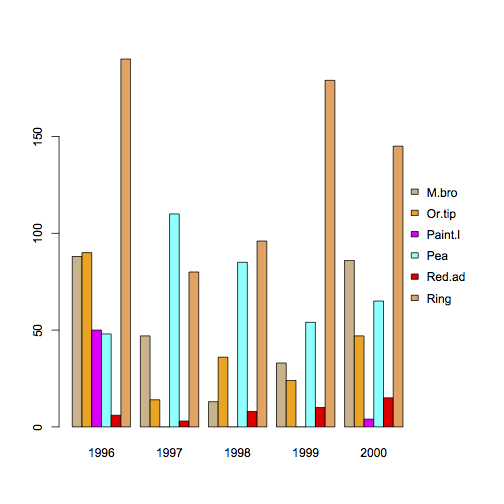
> mycols = c("tan", "orange1", "magenta", "cyan", "red", "sandybrown")
> barplot(bf, beside = TRUE, col = mycols, legend = TRUE, xlim = c(0, 45))
Note that the xlim parameter in this example set the axis from 0 to 45. Each bar in the barplot() takes up a space, so you need to allow about 1 unit per bar plus a bit extra for the legend itself.
Note also that the colparameter set the colors for the plot, which were passed automatically to legend() without requiring the args.legend parameter. Of course if you wanted other parameters (such as supressing the legend box) you would require the args.legend parameter.
Place a legend in a plot margin
Altering the x-axis or y-axis size to accommodate the legend is a fairly simple matter. Sometimes however you want a legend to be at the bottom or even the left, and however you alter the axes you will not make space!
What you need is to be able to place the legend in the margin of the plot, so that it does not overlap the plotting zone at all. To do this you need to tweak the graphical parameters via the par() command.
The general running order is as follows:
- Set the plot margins as you need to give the space in the required margin.
- Make your plot (any plot).
- Reset the graphical parameters back to defaults.
- Now set the plot margins to 0 and at the same time set plotting to allow “overplot”.
- Use legend() to place the legend where your extra-large margin is.
- Reset the graphical parameters back to defaults.
Steps 3 and 6 are not absolutely essential but preferable, as you can get into an awful mess if you forget the current settings.
Legend in the plot margin for a bar chart
To make the plot margin larger use par(oma = c(b, l, t, r)) where b, l, t, r are values for the margin sizes at the bottom, left, top and right. For example:
> opar = par(oma = c(0,0,0,4)) # Large right margin for plot
> mycols = c("tan", "orange1", "magenta", "cyan", "red", "sandybrown")
> barplot(bf, beside = TRUE, col = mycols)
> par(opar) # Reset par
Now you have to set the graphical parameters again, this time set oma, mar and new = TRUE. The last parameter is important as it does not wipe the plot as the graphical parameters are set. Once you’ve altered the graphical parameters you can set the legend():
> opar = par(oma = c(0,0,0,0), mar = c(0,0,0,0), new = TRUE)
> legend(x = "right", legend = rownames(bf), fill = mycols, bty = "n", y.intersp = 2)
> par(opar) # Reset par
Place a legend in the bottom margin of a plot
The bottom margin of a plot can present some slight difficulties because the axis labels get in the way. The easiest solution is to use the inset parameter and shift the legend outwards (use a small negative value).
Start by making space in the bottom outer margin, then make the basic plot:
> opar = par(oma = c(2,0,0,0))
> barplot(bf, beside = TRUE, col = cm.colors(6))
> par(opar) # Reset par
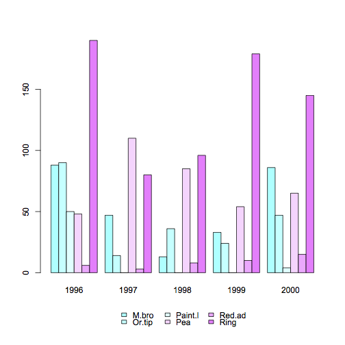
Now set the margins to zero and set the overplot. The legend() command can now be used with the inset parameter:
> opar =par(oma = c(0,0,0,0), mar = c(0,0,0,0), new = TRUE)
> legend(x = "bottom", legend = rownames(bf), fill = cm.colors(6), bty = "n", ncol = 3, inset = -0.15)
> par(opar) # reset par
The inset parameter shifts the legend position slightly, to avoid the axis labels.
Note that positive values for inset shift the position upwards, a value of 0.5 is about half-way up. The direction of the inset shift is determined by the position you set in the command. If you used x = “bottom” then positive values shift the position upwards. If you used x = “right” then positive values shift the position left.
Legend in the plot margin for a scatter or line plot
If you use a line plot or a scatter plot you’ll have to contend with different plotting characters and line types. It is easier to set the parameters explicitly in the plot() command so that they are more easily matched in the legend().
In the following example a matplot() is used to create a multiple-series line plot. The legend is placed in the right margin.
> t(bf) # Rotate the data as matplot() takes columns as series
     M.bro Or.tip Paint.l Pea Red.ad Ring
1996    88     90      50  48      6  190
1997    47     14       0 110      3   80
1998    13     36       0  85      8   96
1999    33     24       0  54     10  179
2000    86     47       4  65     15  145

> mycols = c("tan", "orange1", "magenta", "cyan", "red", "sandybrown")
> opar = par(oma = c(0,0,0,5.5)) # Set right margin

## Plot without axes (because axis labels are numbers)
> matplot(t(bf), ylab = "", type = "b", pch = 1:6, lty = 1:6,
                axes = FALSE, lwd = 2, col = mycols)

> axis(2) # Use default y-axis

# Custom x-axis using years as labels
> axis(1, at = 1:5, labels = colnames(bf))

> box() # Bounding box around plot

> title(ylab = "Abundance", xlab = "Year")
> par(opar) # Reset par

> opar = par(oma = c(0,0,0,0), mar = c(0,0,0,0), new = TRUE)

# Legend pars to match matplot
> legend(x = "right", legend = rownames(bf), col = mycols,
         pch = 1:6, lty = 1:6, bty = "n",
         ncol = 1, text.col = "blue", y.intersp = 2)
> par(opar) # Reset par
Note that in this example the colour of the legend text has also been customized via the text.col parameter. For all the parameters used by legend() type help(legend) into R.

Comments are closed.