Exercise 6.4.2.
Statistics for Ecologists (Edition 2) Exercise 6.4.2
These are some notes about axis labels in R plots, particularly how you can use superscript, bold and so on.
Axis labels in R plots using expression() command
The labelling of your graph axes is an important element in presenting your data and results. You often want to incorporate text formatting to your labelling. Superscript and subscript are particularly important for scientific graphs. You may also need to use bold or italics (the latter especially for species names).
The expression() command allows you to build strings that incorporate these features. You can use the results of expression() in several ways:
- As axis labels directly from plotting commands.
- As axis labels added to plots via the title()
- As marginal text via the mtext()
- As text in the plot area via the text()
You can use the expression() command directly or save the “result” to a named object that can be used later.
Introduction
The expression() command
The expression() command takes regular characters and uses them in a special way, allowing you to build more complicated strings. You don’t need quotes (most of the time) as the usual letters and numbers are not “interpreted”. R usually takes strings that are un-quoted and tries to interpret them as objects or commands.
What the expression() command does do though, is to look for certain characters or phrases, which are treated as “switches” that do something, like turn on superscript or bold font.
- ~ Acts as a space character (actual spaces are ignored in R commands).
- * Acts as a connector, this allows you to join several elements.
- “” Quotes are used to enclose items that would otherwise be treated as a special character (like ~ or *).
So, type a ~ when you want a space and “~” when you want a ~. The * is a connector, which can be used to join sections of the expression. This allows you to “turn off” superscript for example, or switch font face.
There are various “reserved” characters e.g. + – / * ? ^ (mostly they are not letters or numbers), and these should be inside quotes. Items in quotes should be bracketed by ~ and/or * characters.
When you type an expression() any spaces you type are ignored. You can type spaces to help yourself see clearly what you have typed but they are all stripped out. If you display an expression() result R will place a single space (for clarity) between various elements of your expression().
The following expression():
expression(The~"~"~character~forms~spaces)
Would appear like “The ~ character forms spaces” when used in titles or text.
Superscript & subscript
The most common thing you’ll want to do in axis labels is to make superscripts and subscripts.
- ^ Anything following the caret is displayed as superscript.
- [] Anything inside the square brackets is displayed as subscript.
The [] are simple enough to use, anything that you want to be subscripted goes inside the brackets.
Note that you cannot start an expression() with a [ so you have to “fool” the system and use a pair of empty quotes:
expression(""[x]*X)
Note also that if you do that you have to use a connector (*) afterwards (or a space character ~)! The preceding example would produce text like so:
xX
Superscript is “started” by the caret ^ character. Anything after ^ is superscript. The superscript continues until you use a * or ~ character. If you want more text as superscript, then enclose it in quotes. The only exception is + or – when preceded by a number.
In the following example only the word “script” would appear superscript:
expression(Super^script~text)
Superscript text
The following uses quotes to get the two words superscripted.
expression(Super^"script text")
Superscript text
The following commands produce a plot with superscript and subscript labels:
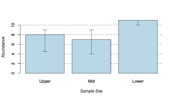
opt = par(cex = 1.5) # Make everything a bit bigger

xl <- expression(Speed ~ ms^-1 ~ by ~ impeller)
yl <- expression(Abundance ~ by ~ Kick ~ net[30 ~ sec] ~ sampling)

plot(abund ~ speed, data = fw, xlab = xl, ylab = yl)

par(opt) # Reset the graphical parameters
The expression() command used to make superscripts and subscripts in axis labels.
Note that R does not “like” subscripts beginning with numbers and continuing with letters! So [2xyz] gives an error but [2 * xyz] is fine.

Font face: bold, italic, underline
You can alter the basic font face by enclosing the items you require in a command-like element:
- plain() Anything in the parentheses is regular plain font face.
- italic()italic.
- bold()Bold
- bolditalic()Italic and bold.
- underline()Underlined.
The font face element must be preceded by a ~ or a * so that R can recognize it as a font face element.
The title() command allows you to specify a general font face as part of the command. Similarly the par() command allows you to specify font face for various plot elements:
- font – the main text font face.
- lab – axis labels.
- main – main title.
- sub – sub-title.
You specify the font face as an integer:
- 1 = Plain.
- 2 = Bold.
- 3 = Italic.
- 4 = Bold & Italic.
You can set the font face(s) from par() or as part of the plotting command. This is useful for the entire label/title but does not allow for mixed font faces. To mix font faces use the expression() elements italic(), bold() and so on.

The following lines give some simple examples:
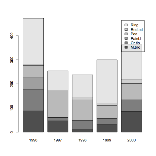
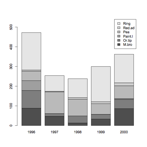
opt <- par(cex = 1.5)

em <- expression(Abundance~of~italic(Gammarus~pulex)plain(~a~shrimp))
ey <- expression(Abundance~30s~underline(kick~sample))
ex <- expression(Speed~bold(ms^-1))

plot(abund ~ speed, data = fw, xlab = ex, ylab = ey, main = em)

par(opt)
To get mixed font faces you need the expression() command.
Note that expression() “does not like” a mix of letters and numbers, so split them using the * character.
Maths expressions
The expression() command can also produce a range of mathematical symbols and… expressions! You can create fractions, degree signs, arrows and all manner of items. These are generally less useful in axis labels but here are a few of the expressions to whet your appetite:
| x + y | Produces x + y. |
| x – y | Produces x – y. |
| x == y | Produces x = y. |
| x != y | Produces x ≠ y. |
| x %~~% y | Produces x ≈ y. |
| x %+-% y | Produces x ± y. |
| x %/% y | Produces x ÷ y. |
| bar(x) | Produces x with an overbar. |
| frac(x, y) | Produces a fraction with x over y. |
| x %up% y | Produces an up arrow, x ↑ y. |
| x %down%y | Produces a down arrow, x ↓ y. |
| x %->% y | Produces a right arrow, x → y. |
| x %<-% y | Produces a left arrow, x ← y. |
| sum(x, a, b) | Produces a sum (capital sigma) symbol, ∑, with optional sub and superscripts. |
| sqrt(x) sqrt(x, y) |
Produces a square root symbol, √x, with optional root, y√x. |
| infinity | An infinity symbol, ∞. |
| alpha – omega | Greek letters in lowercase. |
| Alpha – Omega | Greek letters in uppercase. |
| 180*degree | Produces a degree symbol, 180˚. |
| x ~ y | A space, x y. |
There are plenty of others, type help(plotmath) into your R console to get the help entry page.
Ways to incorporate expression() into plots
There are four main ways you can incorporate expression() objects into your plots:
- In the plot area via text()
- As a title via title()
- Directly via the plotting command; essentially the same as title()
- In the margin via mtext()
As far as the expression() part goes there is no difference between these methods; the main difference is the placement.
Add text to a plot
The text() command allows you to add text, and expression() objects to an existing plot window.
text(x, y, ...)
You need to type in the co-ordinates and then the text, quoted or as an expression(). There are other graphical parameters you can add such as:
col
cex
There are a whole lot more besides, but this article is primarily about axis labels so I’ll gloss over text() for the moment, except to demonstrate some mathematical symbols.
Math symbols
The math symbols can be used in axis labels via plotting commands or title() or as plain text in the plot window via text() or in the margin with mtext().
The following commands place some text into a plot window but the expression() parts would work in axis labels, margins or titles.
opt <- par(cex = 1.5)
plot(1:10, 1:10, type = "n", xlab = "X-vals", ylab = "Y-vals")

text(1, 1, expression(hat(x)))
text(2, 1, expression(bar(x)))
text(2, 2, expression(alpha==x))
text(3, 3, expression(beta==y))
text(4, 4, expression(frac(x, y)))
text(5, 5, expression(sum(x)))
text(6, 6, expression(sum(x^2)))
text(7, 7, expression(bar(x) == sum(frac(x[i], n), i==1, n)))
text(8, 8, expression(sqrt(x)))
text(9, 9, expression(sqrt(x, 3)))

par(opt)
The expression() command used with text() to create math formulae.
You can create quite complicated formulae using expression() but it can also be confusing, especially if you are using a plotting command. Create your expression() first and save the result to a named object to help keep yourself organised.

Add axis titles
You can use the title() command to add titles to the main marginal areas of an existing plot. In general, you’ll use xlab and ylab elements to add labels to the x and y axes. However, you can also add a main or sub title too.
Most graphical plotting commands allow you to add titles directly, the title() command is therefore perhaps redundant. However, it is often easier to set your titles “” (i.e. blank) and then use title() afterwards, especially if they are complicated.
If you are using expression() to make a label/title then save the expression() result as a named object, which is easier to use in the subsequent command(s) that use them.
The title() command has an additional “trick” up its sleeve, the line parameter. This allows you to select a position for the title(s) in lines from the edge of the plot.
- Set line = 0 to place the title beside the axis (where the tick-marks usually are).
- Set line = 1 to place the title one line in (where the axis values usually are).
The maximum value you can set depends on the margin sizes. In practice you can get the margin value minus one. To see the currently set margin sizes:
par(mar)
You’ll get a vector of four values (bottom, left, top, right).
You can also set the title to appear inside the plot using negative values, line = -1 will be adjacent to the axis and just inside.
Add marginal text
The mtext() command allows you to place text and expression() objects into any of the margins of a plot. The mtext() command allows you a bit more control over the placement of the text, compared to the title() command.
The general form of the command is:
mtext(text, side = 3, line = 0, outer = FALSE, at = NA,
      adj = NA, padj = NA, cex = NA, col = NA, font = NA, ...)
| text | The text to write. This can be a character string or an expression. |
| side = 3 | The side of the plot to use. The sides are 1= bottom, 2= left, 3 = top, 4 = right. The default is the top. |
| line = 0 | The line of the margin to use. The default is 0, which is adjacent to the outside of the plot area. Positive values move outward and negative values inward. |
| outer = FALSE | If outer = TRUE, the outer margin is used if available. |
| at = NA | How far along the side to place the text in relation to the axis scale. Text is centered on this point. |
| adj = NA | How far along the side to place the text as a proportion. The default is effectively 0.5, which places the text halfway along. If text is oriented parallel to the axis, adj = 0 will result in left or bottom placement. Text is centered. |
| padj = NA | Adjusts the text perpendicular to the reading direction. This permits “tweaking” of the placement. Positive values place text lower; negative values higher. |
| cex = NA | The character expansion. Values 1 make text larger; values < 1 make text smaller. |
| col = NA | The color for the text. The default, NA, means use the current setting par(“col”). |
| font = NA | The font to use. The default, NA, means use the current setting par(“font”). Use font = 1 for regular text; 2 = bold, 3 = italic, 4 = bold+italic. |
| … | Additional graphics parameters can be used. Of particular interest is las, which controls the text direction:· las = 0—Text parallel to axis (default).
· las = 1—Text horizontal. · las = 2—Text perpendicular to axis. · las = 3—Text vertical. |

The following commands will demonstrate some of the parameters.
Make a basic plot
plot(1:10, 1:10, type = "n", xlab = "x-vals", ylab = "y-vals")
Add marginal text
mtext("mtext(side = 1, line = -1, adj = 1)", side =1, line =-1, adj =1)
mtext("mtext(side = 1, line = -1, adj = 0)", side=1, line=-1, adj=0)
mtext("mtext(side = 2, line = -1, font = 3)", side=2, line=-1, font=3)
mtext("mtext(side = 3, font = 2)", side=3, font=2)
mtext("mtext(side = 3, line = 1, font = 2)", line=1, side=3, font=2)
mtext("mtext(side = 3, line = 2, font = 2, cex = 1.2)", cex=1.2, line=2, side=3, font=2)
mtext("mtext(side = 3, line = -2, font = 4, cex = 0.8)", cex=0.8, font=4, line=-2)
mtext("mtext(side = 4, line = 0)", side=4, line=0)
Using mtext() to place text or expression() objects into plot margins.
The mtext() command allows for fine placement of marginal text. In the example any font face changes were applied directly and the entire text is altered. If you want to have mixed font face then replace the text in quotes with an expression().