Beta coefficients from linear models

Exercise 11.1.2.

Statistics for Ecologists (Edition 2) Exercise 11.1.2

These notes supplement Chapter 11 and explore the use of beta coefficients, which can be a useful addition to a regression analysis.

Beta coefficients from linear models

Introduction

In linear regression your aim is to describe the data in terms of a (relatively) simple equation. The simplest form of regression is between two variables:

y = mx + c

In the equation y represents the response variable and x is a single predictor variable. The slope, m, and the intercept, c, are known as coefficients. If you know the values of these coefficients then you can plug them into the formula for values of x, the predictor, and produce a value for the response.

In multiple regression you “extend” the formula to obtain coefficients for each of the predictors.

y = m1.x1 + m2.x2 + m3.x3 + ... + c

If you standardize the coefficients (using standard deviation of response and predictor) you can compare coefficients against one another, as they effectively assume the same units/scale.

The functions for computing beta coefficients are not built-in to R. In these notes you’ll see some custom R commands that allow you to get the beta coefficients easily. You can download the Beta coeff calc.R file and use it how you like.

What are beta coefficients?

Beta coefficients are regression coefficients (analogous to the slope in a simple regression/correlation) that are standardized against one another. This standardization means that they are “on the same scale”, or have the same units, which allows you to compare the magnitude of their effects directly.

Beta coefficients from correlation

It is possible to calculate beta coefficients more or less directly, if you have the correlation coefficient, r, between the various components:

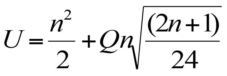
Calculating beta coefficients from correlation coefficients.

The subscripts can be confusing but essentially you can use a similar formula for the different combinations of variables.

Beta coefficients from regression coefficients

In most cases you’ll have calculated the regression coefficients (slope, intercept) and you can use these, along with standard deviation, to calculate the beta coefficients.

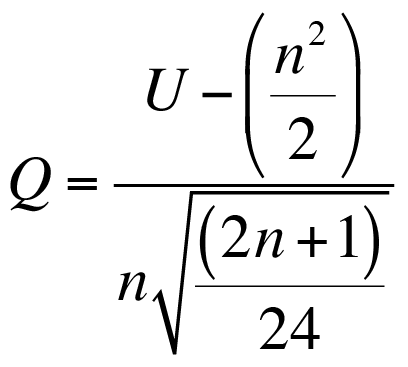
Calculating a beta coefficient from a regression coefficient and standard deviation.

This formula is a lot easier to understand: b’ is the beta coefficient, b is the standard regression coefficient. The x and y refer to the predictor and response variables. You therefore take the standard deviation of the predictor variable, divide by the standard deviation of the response and multiply by the regression coefficient for the predictor under consideration.

There are no built-in functions that will calculate the beta coefficients for you, so I wrote one myself. The command(s) are easy to run/use and I’ve annotated the script/code fairly heavily so it should be useful/helpful for you to see what’s happening.

The beta.coef() command

I wrote the beta.coef() command to calculate beta coefficients from lm() result objects. There are also print and summary functions that help view the results. Here’s a brief overview:

beta.coef(model, digits = 7)
print.beta.coef(object, digits = 7)
summary.beta.coef(object, digits = 7)
model A regression model, the result from lm().
object The result of a beta.coef() command.
digits = 7 The number of digits to display, defaults to 7.


The beta.coef() command produces a result with a custom class beta.coef. The print() and summary() commands will use this class to display the coefficients or produce a more comprehensive summary (compares the regular regression coefficients and the beta).

Using beta.coef()

You will need the result of a linear regression, usually this will be one with the class “lm”.

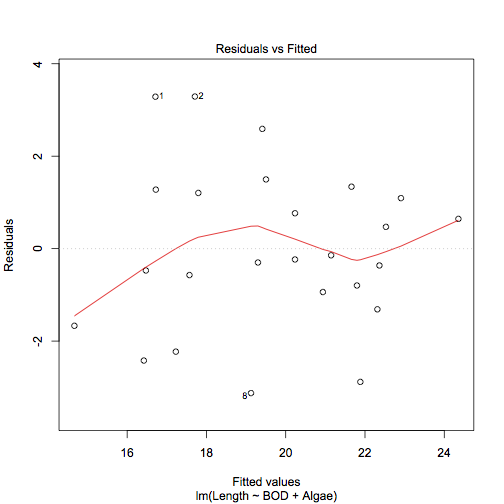
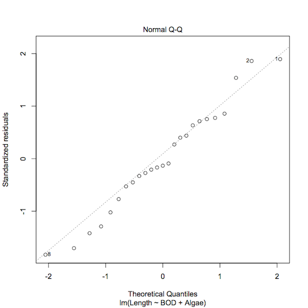
mf.lm <- lm(Length ~ BOD + Algae, data = mf)
summary(mf.lm)

Call:
lm(formula = Length ~ BOD + Algae, data = mf)
Residuals:
 Min      1Q  Median      3Q     Max
-3.1246 -0.9384 -0.2342  1.2049  3.2908
Coefficients:
            Estimate Std. Error t value Pr(>|t|)
(Intercept) 22.34681    4.09862   5.452 1.78e-05 ***
BOD         -0.03779    0.01517  -2.492   0.0207 *
Algae        0.04809    0.03504   1.373   0.1837
Signif. codes:  0 ‘’ 0.001 ‘’ 0.01 ‘’ 0.05 ‘.’ 0.1 ‘ ’ 1
Residual standard error: 1.83 on 22 degrees of freedom
Multiple R-squared:  0.6766,  Adjusted R-squared:  0.6472
F-statistic: 23.01 on 2 and 22 DF,  p-value: 4.046e-06

Once you have the result you can use the beta.coef() command to compute the beta coefficients:

mf.bc <- beta.coef(mf.lm)

Beta Coefficients for: mf.lm
                 BOD     Algae
Beta.Coef -0.5514277 0.3037675

Note that the result is shown even though the result was assigned to a named object.

You can use the print method to display the coefficients, setting the number of digits to display:

print(mf.bc, digits = 4)

Beta coefficients:
              BOD  Algae
Beta.Coef -0.5514 0.3038

The command takes the $beta.coef component from the beta.coef() result object.

Summary beta.coef results

The summary method produces a result that compares the regular regression coefficients and the standardized ones (the beta coefficients). You can set the number of digits to display using the digits parameter:

summary(mf.bc, digits = 5)

Beta coefficients and lm() model summary.
Model call:
lm(formula = Length ~ BOD + Algae, data = mf)
          (Intercept)       BOD    Algae
Coef           22.347 -0.037788 0.048094
Beta.Coef          NA -0.551428 0.303768

The command returns the model call as a reminder of the model.

Add the commands to your version of R

To access the commands, you could copy/paste the code from Beta coeff calc.R. Alternatively, you can download the file and use:

source("Beta coeff calc.R")

As long as the file is in the working directory. Alternatively, on Windows or Mac use:

source(file.choose())

The file.choose() part opens a browser-like window, allowing you to select the file. Once loaded the new commands will be visible if you type ls().

The lm.beta package

After I had written the code to calculate the beta coefficients I discovered the lm.beta package on the CRAN repository.

Install the package:

install.packages("lm.beta")

The package includes the command lm.beta() which calculates beta coefficients. The command differs from my code in that it adds the standardized coefficients (beta coefficients) to the regression model. The package commands also allow computation of beta coefficients for interaction terms.

Use the command:

help(lm.beta)

to get more complete documentation once you have the package installed and running. You can also view the code directly (there is no annotation).

lm.beta
print.lm.beta
summary.lm.beta

The lm.beta() command produces a result with two classes, the original “lm” and “lm.beta”.

Graphing multiple regression

Exercise 11.1.

Statistics for Ecologists (Edition 2) Exercise 11.1

This exercise is concerned with how to produce and chart some diagnostics for regression models (Sections 11.1 and 11.2). The dataset used to illustrate these notes is available as a file: regression diagnostic.csv.

Graphing multiple regression/linear models

Introduction

When you only have two variables (a predictor and a single response) you can use a regular scatter plot to show the relationship. Even if the relationship is logarithmic or polynomial you can represent the situation, as long as there is only one predictor variable.

When you have two or more predictor variables it becomes hard to represent the situation graphically. You can try a 3D plot but they are rarely successful. Generally, you’ll stick to plotting the “most important” predictor variable and display the model as a standard regression table.

However, it can be helpful show some diagnostics from your regression model as graphics. These notes show you how you can produce some simple regression diagnostics and present them graphically.

The data used for these notes can be downloaded as a CSV file: regression diagnostic.csv. The data are the same as shown in the book (mayfly regression) but reproduced here to make it easier to follow the notes.

Fitted values

When you make a regression model you are trying to find the “best” mathematical fit between the variables. In a simple form the relationship will be:

y = mx + c

In this case there is a single predictor variable, x. The m is the slope and c is the intercept. Both m and c are known as coefficients. You might have a logarithmic or polynomial relationship but essentially the form of the relationship is the same:

y = m.log(x) + c
y = ax + bx^2 + c

In multiple regression you have more than one predictor and each predictor has a coefficient (like a slope), but the general form is the same:

y = ax + bz + c

Where a and b are coefficients, x and z are predictor variables and c is an intercept. You can add more and more variables:

y = m1.x1 + m2.x2 + m3.x3 + ... + c

Note that each predictor variable has a unique coefficient.

Once you have your “equation” you can use the observed values of the predictors and of the coefficients in your equation to produce new y-values. These values are “fitted” to the regression model. Think of them as being idealised values or “expected” values.

Note that you should not call these fitted values “predicted” values because they are based on your observed predictor variable values. If you insert predictor values that you did not observe into the equation, then you can call the resulting y-values predicted y-values. The values you insert to the equation could lie within the max-min range of observed predictor (interpolation) or be outside (extrapolation). In general, it is “safer” to go with interpolation than with extrapolation.

Calculate Fitted values using R

Fitted values are easy to compute in R. You can get them from the result of a lm() command in two ways:

model$fitted.values
fitted(model)

In both cases model is the result of a lm() command.

names(mf)
[1] "Length" "Speed" "Algae" "NO3" "BOD"
mf.lm = lm(Length ~ BOD + Algae, data = mf)

Then you can get the fitted values:

fitted(mf.lm)
1        2        3        4        5        6        7        8
16.71301 17.70924 19.40969 21.65981 21.79722 20.93840 21.88309 19.12458
9       10       11       12       13       14       15       16
17.22829 16.42101 19.50246 20.23417 21.14452 20.23417 17.79511 16.72331
17       18       19       20       21       22       23       24
17.57183 19.29977 22.31250 14.66902 16.47254 24.35649 22.90681 22.52893
25
22.36403

Once you have the values you can use them like any other numeric variable (the vector has a names attribute).

Calculate Fitted values using Excel

To get fitted values in Excel you’ll need to calculate the coefficients and plug the values into the spreadsheet to generate them:

  1. Arrange your data so that the predictor values are next to one another.
  2. Use the LINEST function to determine the coefficients:
    1. Highlight one block of cells in a row, you need one cell per coefficient.
    2. Type =LINEST and start the formula, inside the () you need
    3. The y-values, the x-values, 1, 0. Note that the final 0 suppresses additional regression stats, you only get the coefficients.
    4. Enter the formula as an array using Control+Enter
  3. The results of LINEST show the coefficients backwards! The intercept is last. The first coefficient shows the last of the predictor variables.
  4. Use the coefficient values and the observed predictors to make your predicted values.

Once you have the coefficients it is fairly easy to create the fitted values but you will need to “fix” the references to the coefficients using $ in the cell reference(s). Then you can copy/paste the formula down the column to fill in the fitted values for all the rows of data.

Use the Analysis ToolPak

If you have the Analysis ToolPak add-in you can use this to generate the regression statistics. The Regression routine will produce the coefficients as well as the fitted values.

  1. Arrange your data so that the predictor values are next to one another.
  2. Click the Data > Data Analysis
  3. Select the Regression option.
  4. Use the mouse to select the appropriate data (you can include the label headings).
  5. Choose the location for the results, which can be in the current worksheet or in another.
  6. Tick the box labelled, Residuals.
  7. Click OK to finish.

Residuals

Residual values are the difference between the fitted values and the actually observed values for your response variable. Think of the fitted values as being the “ideal” or “expected” values based on your regression equation. The residual values are (usually) not ideal and differ from the “perfect fit”.

So, the residuals are a way to see how bad the fit is between the ideal values based on your regression model and the real situation. In general, you want to see that the residuals are normally distributed, at least this is what you want when doing regular linear regression (and curvilinear). In diagnostic terms it is the normal distribution of the residuals that is the really important thing, not the distribution of the original data (although usually you do not get the former without the latter).

Calculate residuals using R

Residual values are easy to compute using R; you get them from the result of a lm() command:

model$residuals
resid(model)

Simply make your regression model result then away you go:

mf.lm = lm(Length ~ BOD + Algae, data = mf)

fitted(mf.lm)
1        2        3        4        5        6        7        8
16.71301 17.70924 19.40969 21.65981 21.79722 20.93840 21.88309 19.12458
9       10       11       12       13       14       15       16
17.22829 16.42101 19.50246 20.23417 21.14452 20.23417 17.79511 16.72331
17       18       19       20       21       22       23       24
17.57183 19.29977 22.31250 14.66902 16.47254 24.35649 22.90681 22.52893
25
22.36403

The result of resid() is a numerical vector (with a names attribute), which you can use in various ways (as you will see later).

Calculate residuals using Excel

Residuals are simply the difference between the observed and expected values of your response variable. You can use the regression equation for your model to generate the fitted values. Once you have those you simply subtract the fitted value from the observed:

Observed – Fitted = Residual

Note that you always carry out the calculation this way around by convention.

Use the Analysis ToolPak

The Analysis ToolPak can compute the residuals for you easily. You simply tick the box labelled Residuals in the Regression dialogue box. The process is exactly the same as when calculating the fitted values.

The residuals are placed alongside the fitted values (which are labelled Predicted), and are labelled Residuals.

Standardized residuals

Standardized residuals are residuals that have been rescaled. The way they are scaled is such that each residual value has unit standard deviation. The standardization process takes into account how much “influence” a datum might have on the regression (something called leverage).

It is generally preferable to use the standardized residuals.

Standardized residuals in R

You can compute the standardized residuals using the rstandard() command:

rstandard(mf.lm)
1           2           3           4           5           6
1.89433577  1.85925744  1.53830120  0.77572446 -0.45212719 -0.52806189
7           8           9          10          11          12
-1.70410540 -1.82866111 -1.29005538 -1.41946426  0.85656348  0.43789841
13          14          15          16          17          18
-0.09180616 -0.13389770  0.71314102  0.75324789 -0.32958291 -0.16844397
19          20          21          22          23          24
-0.76996058 -1.02235369 -0.27307270  0.39957434  0.63390452  0.27061395
25
-0.20911178

The result is a numeric vector (with a names attribute).

Standardized residuals in Excel

You cannot calculate the standardized residuals in Excel without some tedious computations! The Analysis ToolPak claims to calculate standardized residuals but what you end up with is the residuals divided by the standard deviation of the residuals. This is only an approximation to the “proper” standardization.

Diagnostic plots

There are several type of plot you might use as diagnostic tools. The ones I’ll show here are:

  • Residuals vs. Fitted values.
  • Normal distribution plot of standardized residuals.

You can make these plots easily using R. In Excel you can make some worthwhile attempts but you can only use approximately standardized residuals.

Residuals vs. Fitted values

You can calculate the fitted and residuals easily in R or Excel. A plot of the residuals against the fitted values is a simple way to produce a useful diagnostic tool.

Plot using R

The simplest way to produce a residual plot is to use the plot() command on a regression model result (which actually runs the plot.lm() command). The plot.lm() command produces up to six diagnostic plots, which you can choose using the which = parameter. The plot of residuals vs. fitted values is obtained via:

plot(model, which = 1)

This produces a scatter plot of the regular residuals against the fitted values. The command also produces a locally weighted polynomial smooth fit line and identifies and data points that might have undue influence on the model fit.

plot(mf.lm, which = 1)

Ideally you would like not to see any kind of pattern. In the example there are some points identified as possibly having undue influence but the lowess line runs aimlessly along the middle.

You can produce a similar plot using standardized residuals and regular plot commands:

plot(fitted(mf.lm), rstandard(mf.lm))
abline(h = 0, lty = 3)
lines(lowess(fitted(mf.lm), rstandard(mf.lm)), col = "red")
Plot using Excel

It is fairly easy to plot the regular residuals against the fitted values using Excel. Once you have calculated the values you can simply make a scatter plot. However, it is not so easy to add a locally weighted polynomial. There are add-ins you might try but a simple workaround is to use a moving average trendline. To incorporate this, you need to sort the fitted values in ascending numerical order.

  1. First of all, you need to calculate the fitted values and the residuals. You can do this using the Analysis ToolPak.
  2. If you used regular commands to compute the values, then:
    1. Copy them to the clipboard.
    2. Paste Special the values only to a new location.
  3. If you used the Analysis ToolPak you do not need to do anything.
  4. Highlight the values (include their headings) and sort them:
    1. Click the Home > Sort & Filter button.
    2. Click Custom Sort.
    3. Use the dropdown on the left to sort by the Fitted values.
    4. Make sure you use Smallest to Largest.
    5. Click OK to apply the sort.
  5. Now you have the fitted values sorted in ascending numerical order.

Make a scatter plot by highlighting the fitted and residual values data (and the column headings). You want to ensure that the fitted values are in the first column (Excel will expect this).

Add a moving average trendline.

  • In Excel 2013 click the chart then use the Design > Add Chart Element
  • In Excel 2010 click the chart then use the Layout > Trendline

You want to select the Moving Average option. The default is for a two-point moving average. This is okay for some cases and not for others so format the trendline and alter the options until you get something that looks sensible. In the following chart a 4-point moving average was used.

A residual vs. fitted values plot in Excel. Use a moving point average trendline to get an impression of the fit (or lack of).

The moving average trendline is not a perfect solution but it will give you an idea.

Distribution plot of residuals

Ideally you want the residuals (standardized) to be normally distributed. In R you can calculate the standardized residuals and plot a histogram or QQ plot to show the distribution. In Excel you can only approximate the standardized residuals, which you can plot as a histogram or a QQ plot (with a bit of work).

Plot using R

The simplest solution is to use plot() on the result of a regression model. If you use the parameter, which = 2, you’ll get a QQ plot of the standardized residuals.

plot(mf.lm, which = 2)

A normal QQ plot of the standardized residuals of a regression model.

You can see that the plot() command has highlighted those data points that have some influence over the model fit. You can produce a similar plot using regular commands:

qqnorm(rstandard(mf.lm))
qqline(rstandard(mf.lm), lty = 3)

However, this would not identify any “odd points”.

Plot using Excel

Once you have the residuals in Excel (either by direct calculation or via the Analysis ToolPak) you are well on your way to making a normal distribution plot. If you want the standardized residuals you will have to put up with Excel’s approximation. You can work out the approximate values using:

Approx Std.Resid = Residual / Stdev(Residual)

Or let the Analysis ToolPak calculate this for you.

You can then make a histogram of the values. You’ll have to select appropriate bins and use the FREQUENCY function to work out the frequencies. Alternatively, you can let the Analysis ToolPak work out frequencies for you via the Histogram routine (which will make the chart too).

It is possible to produce a QQ plot, which requires a few steps:

  1. Make a column of “ranks”, which is a simple list of “observation number”, values from 1 to the number of replicates (rows) in your dataset.
  2. Now determine the cumulative proportion for the rank values. You need a formula resembling: =(rank-0.5)/count(rank1:rankn) where rank1:rankn is your column of rank values and rank is the rank you are working out the proportion of. You will need to “fix” the cell references for rank1:rankn using $.
  3. Copy and paste the formula down the column. You should see ascending values rising towards a value of 1 (you’ll probably end up with 0.98).
  4. In the next column you need to calculate a z-score. Use NORMSINV to work this out using the proportions you just calculated. You should end up with a series of values starting at about -2 and rising through 0 to around +2.
  5. In the next column copy your standardized residual values.
  6. Sort the residuals from smallest to largest.
  7. Highlight the z-score and sorted residuals data.
  8. Insert a Scatter plot.

You can add a linear trendline and with a bit of formatting can end up with a half decent QQ plot.

A QQ plot of residuals from a regression model.

The QQ plot is a bit more useful than a histogram and does not take a lot of extra work. However, it can be a bit tedious if you have many rows of data.

Post-hoc testing in Kruskal-Wallis using R

Exercise 10.2.3.

Statistics for Ecologists (Edition 2) Exercise 10.2.3

These notes are about post hoc analysis when you use the non-parametric Kruskal-Wallis test. They supplement Chapter 10 in relation to using R to calculate differences between >2 non-parametric samples.

Post-hoc testing in the Kruskal-Wallis test using R

Introduction

The Kruskal-Wallis test is a non-parametric test for differences between more than two samples. It is essentially an analogue for a one-way anova. There is no “standard” method for carrying out post hoc analysis for KW tests. These notes show you how you can use a modified form of the U-test to carry out post hoc analysis.

When you carry out a Kruskal-Wallis test you are looking at the ranks of the data and comparing them. If the ranks are sufficiently different between samples you may be able to determine that these differences are statistically significant.

However, the main analysis only tells you about the overall situation, the result tells you that “there are differences”. Look at the following graph, which shows three samples.

A Kruskal-Wallis test of these data gives a significant result, H = 6.54 p < 0.05, but does not give any information about the pair by pair comparisons. Looking at the graph you might suppose that the Upper and Mid samples are perhaps not significantly different as their error bars (IQR) overlap considerably. The Lower sample appears perhaps to be different from the other two.

The way to determine these pairwise differences is with a post hoc test. You cannot simply carry out regular U-tests because you’ll need to carry out at least 3 and this “boosts” the chances of you getting a significant result by a factor of 3. You could simply adjust the p-values (e.g. using a Bonferroni correction), but this is generally too conservative.

These notes show you how to carry out a modified version of the U-test as a post hoc tool. The approach is analogous to the Tukey HSD test you’d use with parametric data.

A modified U-test as a post-hoc tool

With a bit of tinkering you can modify the formula for the U test to produce the following:

A critical value for U in a post hoc test for Kruskal-Wallis. Q is the Studentized range and n the harmonic mean of sample sizes.

In the formula n is the harmonic mean of the sample sizes being compared. and Q is the value of the Studentized Range for df = Inf, and number of groups equal to the original number of samples.

Critical values of Q, the Studentized range.

Number of
groups
Significance
5% 1%
2 2.772 3.643
3 3.314 4.120
4 3.633 4.403
5 3.858 4.603
6 4.030 4.757


The formula calculates a critical U-value for the pairwise comparison. You simply carry out a regular U-test, then use the largest U-value as a test statistic. If your value is equal or larger than the critical value from the formula, then the pairwise comparison is a statistically significant one.

Harmonic mean

The harmonic mean is easy to determine:

Calculating the harmonic mean of two values.

The harmonic mean is a way of overcoming differences in sample size. The more different the sample sizes the more unreliable this approach will be.

Calculate Q directly

If you re-arrange the formula you can calculate a value for Q:

Calculate a value for Q (Studentized range) from the result of a U-test.

You can now use the result of a U-test (use the larger of the two calculated U-values) to work out a value for Q. Now you can compare your Q-value to the critical value.

The Studentized range is a distribution built into the basic R program. This gives you a way to compute an exact p-value for the pairwise comparison.

Custom R functions for Kruskal-Wallis post hoc

I’ve produced four custom functions for use with Kruskal-Wallis post hoc tests:

  • mean() – Calculates the harmonic mean of two values.
  • post() – Calculates the post hoc results for a pairwise comparison of two samples from a larger dataset.
  • post() – Calculates the exact p-value for a post hoc given a U-value, number of groups and sample sizes.
  • post() – Calculates a critical U-value for a post hoc given a confidence level (default 95%), number of groups and sample sizes.

These functions are contained in a single file: KW posthoc.R. If you source() the file you will set-up the functions and see a message giving some idea of what the functions do.

The h.mean() function

h.mean(n1, n2)
n1, n2 Numerical values representing sample sizes of two samples.


This function simply returns the harmonic mean of two numbers, i.e. the sample sizes of two samples.

h.mean(5, 7)
[1] 5.833333

The function is called by the other post hoc functions (and is built-in) but it might be “handy” to have separately.

The KW.post() function

KW.post(x, y, data)
x, y Numeric samples to compare.
data The data object that contains the samples. It is assumed that the data is in sample format with multiple columns, each representing a separate sample.


The function returns several results as a list:

  • uval – The calculated U value for the pairwise comparison (the larger of the two calculated values).
  • crit – The critical U value at 95%.
  • value – The exact probability for the pairwise comparison.

The function also displays the results to the console, even if you assign the result to a named object.

hog3
  Upper Mid Lower
1     3   4    11
2     4   3    12
3     5   7     9
4     9   9    10
5     8  11    11
6    10  NA    NA
7     9  NA    NA

KW.post(Upper, Lower, data = hog3)

Data:  hog3
Pairwize comparison of:  Upper  and  Lower
U-value:  32.5
U-crit (95%):  31.06011
Post-hoc p-value:  0.02641968

If your data are in scientific recording layout, that is you have a response variable and a predictor variable, then you need a slightly different approach. You’ll have to work out a U-test result first, then run the KWp.post() and/or KWu.post() commands (see below).

The KWp.post() function

KWp.post(Uval, grp, n1, n2)
Uval A calculated U-value for the pairwise comparison (the larger of the two calculated values).
grp The number of groups (samples) in the original Kruskal-Wallis test.
n1, n2 The sample sizes of the two groups being analysed.


This function returns an exact p-value for a post hoc analysis. The value is returned immediately.

KWp.post(18, grp = 3, 7, 5)
Post-hoc p-value: 0.9851855

You can carry out a wilcox.test() on two samples to obtain a U-value. You need to know samples sizes because you need the larger of the two U values.

The wilcox.test() only gives one value so you must work out if the value you got was the largest. It so happens that:

n1 * n2 = U1 + U2

This means that you can work out the alternative U-value easily if you know sample sizes.

If your data are in recording layout, with a predictor and response, you’ll need to use the subset parameter to carry out the pairwise test:

hog2
   count  site
1      3 Upper
2      4 Upper
3      5 Upper
4      9 Upper
5      8 Upper
6     10 Upper
7      9 Upper
8      4   Mid
9      3   Mid
10     7   Mid
11     9   Mid
12    11   Mid
13    11 Lower
14    12 Lower
15     9 Lower
16    10 Lower
17    11 Lower

wilcox.test(count ~ site, data = hog2, subset = site %in% c("Upper", "Lower"))

Wilcoxon rank sum test with continuity correction
data:  count by site
W = 32.5, p-value = 0.01732
alternative hypothesis: true location shift is not equal to 0

Check the sample sizes:

replications(count ~ site, data = hog2)

$site
site
Lower   Mid Upper
    5     5     7

Now you can see if the U-value you got was the largest:

5*7 – 32.5
[1] 2.5

Since it is the largest, you can use it in the KWp.post() function:

KWp.post(32.5, grp = 3, 5, 7)

Post-hoc p-value: 0.02641968

Generally speaking the wilcox.test() will return the largest U-value if you use the response ~ predictor format for the command. If you run the command on separate samples the returned U-value will depend on the order you specify the samples.

The KWu.post() function

KWu.post(CI = 0.95, grp, n1, n2)
CI = 0.95 The confidence interval, defaults to 0.95. This is essentially a significance level of p = 0.05.
grp The number of groups (samples) in the original Kruskal-Wallis test.
n1, n2 The sample sizes of the two groups being analysed.


This function returns a U-value for a given confidence level. You supply the number of groups (samples) in the original Kruskal-Wallis test and the sizes of the two samples being compared. The result is a critical value, which means you can carry out the wilcox.test() and compare the resulting U-value to this critical value.

KWu.post(CI = c(0.95, 0.99), grp = 3, n1 = 5, n2 = 5)
Post-hoc critical U value:    23.71961 26.44729

In the example you see that you can set multiple confidence intervals. Here the critical U values for p = 0.05 and p = 0.01 are returned.

Adjustment for tied ranks in the Kruskal-Wallis test

Exercise 10.2.b.

Statistics for Ecologists (Edition 2) Exercise 10.2.b

These notes are concerned with the Kruskal-Wallis test (Section 10.2). The notes show you how to adjust your test statistic when you have tied values, and so tied ranks.

Adjusting for tied ranks in the Kruskal-Wallis test

Introduction

The Kruskal-Wallis test is appropriate when you have non-parametric data and one predictor variable (Section 10.2). It is analogous to a one-way ANOVA but uses ranks of items in various groups to determine the likely significance.

When you have tied values, you will get tied ranks. In these circumstances you should apply a correction to your calculated test statistic. The notes show you how this can be done. The calculations are simple but in Excel it can be difficult to get the process “automated”. In R the kruskal.test() command computes the adjustment for you.

Calculating the adjustment factor

In order to correct for tied ranks you first need to know which values are tied. Then you need to know how many ties there are for each rank value. Finally, you’ll need to know how many replicates there are in the dataset.

Once you’ve ascertained these things you can use the following formula to work out a correction, or adjustment, factor:

In the formula t is the number of ties for each rank value. For each value of t, you evaluate the t-cubed minus t part. This is then summed for all the tied values (values without ties can also be evaluated but 13 – 1 = 0). Once you have the numerator you work out the denominator using n, the number of replicates in the original dataset.

The final value of D is then 1 – your fraction.

Adjusting the KW test statistic

Once you have the value of D, the correction factor, you can use it to adjust the original Kruakal-Wallis test statistic (H).

Formula for adjustment of the Kruskal-Wallis statistic in the case of tied ranks.

The correction is simple: H/D.

You then use the Hadj value in place of the original to determine the final test significance (using critical values tables – see exercise 10.2a).

Example data

Have a look at the correction in action using the following example:

Example data. Three non-parametric samples for use in Kruskal-Wallis test.

Upper Mid Lower
3 4 11
4 3 12
5 7 9
9 9 10
8 11 11
10
9


Here there are three samples and you can see that there are tied values, so you know there will be tied ranks.

Example ranks

The first step is to evaluate the ranks. Each value is replaced by its rank in the overall dataset.

Sample data shown as ranks instead of original values. Samples are combined for ranking.

Upper Mid Lower
1.5 3.5 15
3.5 1.5 17
5 6 9.5
9.5 9.5 12.5
7 15 15
12.5
9.5


The Kruskal-Wallis test looks at the sum of the ranks from each sample. If the ∑rank is different between samples there is a good chance that differences are statistically significant. If the ∑rank are close, then differences are less likely to be significant.

In this example the rank sums are:

Rank sums for three samples.

Upper Mid Lower
48.5 35.5 69


You can now calculate the Kruskal-Wallis test statistic, H.

Original H value

Once you have the rank sums you can compute the Kruskal-Wallis test statistic:

Formula for calculating the Kruskal-Wallis statistic for non-parametric samples.

The Kruskal–Wallis formula looks pretty horrendous but actually it is not that bad. The numbers 12 and 3 are constants. Uppercase N is the total number of observations. The R refers to the ranks of the observations in each sample and n is the number of observations per sample.

In the example the final value of the Kruskal-Wallis statistic works out to be H = 6.403.

Tied ranks

The formula for working out the correction factor was given earlier. You need to work out, for each rank value, the number of repeats.

It is not easy to do this “automatically” using Excel. There are ways you could make a template to evaluate the ties for you but it is complicated. Since you can do it using a bit of copy and paste, this is what you’ll see here.

Start by assembling the ranks into a single column. This means a bit of copy and paste but you’ll probably need to use Paste Special to place the Values only.

When you paste the ranks you only want the numbers and don’t want the formula (which would give an error).

Once you have the column of ranks you can simply re-arrange them in ascending order (use the Home > Sort & Filter button or the Data > Sort button). In the following table the second column shows the sorted ranks (you don’t need to make a second column, I have done this to show the effect).

Rearranging ranked data to make calculation of tied ranks easier.

Rnk Ord Ties T3-T
1.5 1.5
3.5 1.5 2 6
5 3.5
9.5 3.5 2 6
7 5
12.5 6
9.5 7
48.5 9.5
3.5 9.5
1.5 9.5
6 9.5 4 60
9.5 12.5
15 12.5 2 6
17 15
9.5 15
12.5 15 3 24
15 17
15 48.5


Once you have the ranks in order it is easy to work out the number of repeats by inspection. You can simply fill in the values as you work down the column. In the preceding table the 3rd column shows the tied rank repeats. So, for example the rank 1.5 is repeated 2 times. The rank 9.5 has 4 repeats.

The final column shows the T3 – T values. In other words, you take the number of repeats and cube it, then subtract the number of repeats.

Once you have these values you can sum them to get an overall value, in this case 102.

Final H adjustment

Once you have your final sum of T3 -3 values you can work out the value of D using the formula given earlier. You need to know the total number of replicates in the original dataset (in this case 17).

The final value of D works out at: 0.9792.

The adjusted H value is then H/D = 6.403 / 0.9792 = 6.540.

You can now use the adjusted H-value to compare to critical value tables (see exercise 10.2a) to see if your result is statistically significant.

(more…)

Critical values for the Kruskal-Wallis test

Exercise 10.2.a.

Statistics for Ecologists (Edition 2) Exercise 10.2a

These notes are concerned with the Kruskal-Wallis test (Section 10.2). The notes give the critical values for the Kruskal-Wallis test under various scenarios.

Critical values for the Kruskal-Wallis test

Introduction

The Kruskal-Wallis test is appropriate when you have non-parametric data and one predictor variable (Section 10.2). It is analogous to a one-way ANOVA but uses ranks of items in various groups to determine the likely significance.

If there are at least 5 replicates in each group, the critical values are close to the Chi-Squared distribution. There are exact critical values computed when you have equal group sizes. There are also exact critical values for situation where you have un-equal group sizes.

General critical values: sample sizes >= 5

When you have at least 5 observations in each group the Kruskal-Wallis critical value is approximately the same as Chi Squared. You need to determine the degrees of freedom, which are the number of groups minus 1. You can reject the null hypothesis if your calculated value of H is bigger than the tabulated value.

Critical values for H where all samples have at least 5 replicates.

degrees of Significance level
freedom 5% 2% 1% 0.01%
1 3.841 5.412 6.635 10.830
2 5.991 7.824 9.210 13.820
3 7.815 9.837 11.341 16.270
4 9.488 11.668 13.277 18.470
5 11.070 13.388 15.086 20.510
6 12.592 15.033 16.812 22.460
7 14.067 16.622 18.475 24.320
8 15.507 18.168 20.090 26.130
9 16.909 19.679 21.666 27.880
10 18.307 21.161 23.209 29.590
11 19.675 22.618 24.725 31.260
12 21.026 24.054 26.217 32.910
13 22.362 25.472 27.688 34.530
14 23.685 26.873 29.141 36.120
15 24.996 28.259 30.578 37.700
16 26.296 29.633 32.000 39.250
17 27.587 30.995 33.409 40.790
18 28.869 32.346 34.805 42.310
19 30.144 33.687 36.191 43.820
20 31.410 35.020 37.566 45.310
21 32.671 36.343 38.932 46.800
22 33.924 37.659 40.289 48.270
23 35.172 38.968 41.638 49.730
24 36.415 40.270 42.980 51.180
25 37.652 41.566 44.314 52.620
26 38.885 42.856 45.642 54.050
27 40.113 44.140 46.963 55.480
28 41.337 45.419 48.278 56.890
29 42.557 46.693 49.588 58.300
30 43.773 47.962 50.892 59.700

Exact values: Equal sample sizes

If you have the same number of replicates for each group you can use a table of exact values, instead of the Chi Squared approximation. There are separate tables for different numbers of groups. Reject the null hypothesis if your calculated value of H is equal or greater than the tabulated value for the appropriate sample size.

Groups = 3

Significance level
Sample 5% 2% 1%
size Groups = 3
2
3 5.600 6.489 7.200
4 5.692 6.962 7.654
5 5.780 7.220 8.000
6 5.801 7.240 8.222
7 5.819 7.332 8.378
8 5.805 7.355 8.465
9 5.831 7.418 8.529
10 5.853 7.453 8.607
11 5.885 7.489 8.648
12 5.872 7.523 8.712
13 5.901 7.551 8.735
14 5.896 7.566 8.754
15 5.902 7.582 8.821
16 5.909 7.596 8.822
17 5.915 7.609 8.856
18 5.932 7.622 8.865
19 5.923 7.634 8.887
20 5.926 7.641 8.905
21 5.930 7.652 8.918
22 5.932 7.657 8.928
23 5.937 7.664 8.947
24 5.936 7.670 8.964
25 5.942 7.682 8.975
infinity 5.991 7.824 9.210

Groups = 4

Exact critical values for H for four groups of equal size.

Significance level
Sample 5% 2% 1%
size Groups = 4
2 6.167 6.667 6.667
3 7.000 7.872 8.538
4 7.235 8.515 9.287
5 7.377 8.863 9.789
6 7.453 9.027 10.090
7 7.501 9.152 10.250
8 7.534 9.250 10.420
9 7.557 9.316 10.530
10 7.586 9.376 10.620
11 7.623 9.422 10.690
12 7.629 9.458 10.750
13 7.645 9.481 10.800
14 7.658 9.508 10.840
15 7.676 9.531 10.870
16 7.678 9.550 10.900
17 7.682 9.568 10.920
18 7.698 9.583 10.950
19 7.701 9.595 10.980
20 7.703 9.606 10.980
21 7.709 9.623 11.010
22 7.714 9.629 11.030
23 7.719 9.640 11.030
24 7.724 9.652 11.060
25 7.727 9.659 11.070
infinity 7.815 9.837 11.340

Groups = 5

Exact critical values for H for five groups of equal size.

Significance level
Sample 5% 2% 1%
size Groups = 5
2 7.418 8.073 8.291
3 8.333 9.467 10.200
4 8.685 10.130 11.070
5 8.876 10.470 11.570
6 9.002 10.720 11.910
7 9.080 10.870 12.140
8 9.126 10.990 12.290
9 9.166 11.060 12.410
10 9.200 11.130 12.500
11 9.242 11.190 12.580
12 9.274 11.220 12.630
13 9.303 11.270 12.690
14 9.307 11.290 12.740
15 9.302 11.320 12.770
16 9.313 11.340 12.790
17 9.325 11.360 12.830
18 9.334 11.380 12.850
19 9.342 11.400 12.870
20 9.353 11.410 12.910
21 9.356 11.430 12.920
22 9.362 11.430 12.920
23 9.368 11.440 12.940
24 9.375 11.450 12.960
25 9.377 11.460 12.960
infinity 9.488 11.670 13.280

Groups = 6

Exact critical values for H for six groups of equal size.

Significance level
Sample 5% 2% 1%
size Groups = 6
2 8.846 9.538 9.846
3 9.789 11.030 11.820
4 10.140 11.710 12.720
5 10.360 12.070 13.260
6 10.500 12.330 13.600
7 10.590 12.500 13.840
8 10.660 12.620 13.990
9 10.710 12.710 14.130
10 10.750 12.780 14.240
11 10.760 12.840 14.320
12 10.790 12.900 14.380
13 10.830 12.930 14.440
14 10.840 12.980 14.490
15 10.860 13.010 14.530
16 10.880 13.030 14.560
17 10.880 13.040 14.600
18 10.890 13.060 14.630
19 10.900 13.070 14.640
20 10.920 13.090 14.670
21 10.930 13.110 14.700
22 10.940 13.120 14.720
23 10.930 13.130 14.740
24 10.930 13.140 14.740
25 10.940 13.150 14.770
infinity 11.070 13.390 15.090

Exact values: Unequal sample sizes

When you have different sample sizes you can look up exact critical values using the following table(s).

Max group size = 1 to 5

The sample sizes are given in the first column, so 222110 is equivalent to 5 groups with replicates of 2, 2, 2, 1 and 1. Reject the null hypothesis if your calculated value of H is equal or greater than the tabulated value.

Critical values of H for unequal group sizes (max replicates 5).

Sample Significance level
sizes 5% 2% 1%
222110 6.750
222111 7.600 7.800
222200 6.167 6.667 6.667
222210 5.679
222210 7.133 7.533 7.533
222211 8.018 8.455 8.618
222220 7.418 8.073 8.291
222221 8.455 9.000 9.227
222222 8.846 9.538 9.846
311100
311111
321100
321110 6.583
321111 7.467
322000 4.714
322100 5.833 6.500
322110 6.800 7.400 7.600
322111 7.954 8.345 8.509
322200 6.333 6.978 7.133
322210 7.309 7.836 8.127
322211 8.348 8.939 9.136
322220 7.682 8.303 8.682
322221 8.731 9.346 9.692
322222 9.033 9.813 10.220
331000 5.143
331100 6.333
331110 7.111 7.467
331111 7.909 8.564 8.564
332000 5.361 6.250
332100 6.244 6.689 7.200
332110 7.200 7.782 8.073
332111 8.303 8.803 9.045
332200 6.527 7.182 7.636
332210 7.591 8.258 8.576
332211 8.615 9.269 9.628
332220 7.910 8.667 9.115
332221 8.923 9.714 10.150
333000 5.600 6.489 7.200
333100 6.600 7.109 7.400
333110 7.576 8.242 8.424
333111 8.641 9.205 9.564
333200 6.727 7.636 8.015
333210 7.769 8.590 9.051
333211 8.835 9.670 10.080
333220 8.044 9.011 9.505
333300 7.000 7.872 8.538
333310 8.000 8.879 9.451
411000
411111 7.333
421000
421100 5.833
421110 6.733 7.267
421111 7.827 8.236 8.400
422000 5.333 6.000
422100 6.133 6.667 7.000
422110 7.145 7.636 7.936
422111 8.205 8.727 9.000
422200 6.545 7.091 7.391
422210 7.500 8.205 8.545
422211 8.558 9.192 9.538
422220 7.846 8.673 9.077
422221 8.868 9.643 10.070
431000 5.208
431100 6.178 6.711 7.067
431110 7.073 7.691 8.236
431111 8.053 8.758 9.023
432000 5.444 6.144 6.444
432100 6.309 7.018 7.455
432110 7.439 8.091 8.394
432111 8.429 9.115 9.506
432200 6.621 7.530 7.871
432210 7.679 8.545 8.962
432211 8.742 9.577 10.010
432220 7.984 8.918 9.429
433000 5.791 6.564 6.745
433100 6.545 7.485 7.758
433110 7.660 8.513 8.891
433111 8.654 9.495 9.934
433200 6.795 7.763 8.333
433210 7.874 8.830 9.374
433300 6.984 7.995 8.659
441000 4.967 6.667 6.667
441100 5.945 7.091 7.909
441110 7.114 8.182 8.636
441111 8.231 9.096 9.538
442000 5.455 6.600 7.036
442100 6.386 7.364 7.909
442110 7.500 8.385 8.885
442111 8.571 9.445 9.940
442200 6.731 7.750 8.346
442210 7.797 8.802 9.330
443000 5.598 6.712 7.144
443100 6.635 7.660 8.231
443110 7.714 8.742 9.247
443200 6.874 7.951 8.621
443300 7.038 8.181 8.876
444000 5.692 6.962 7.654
444100 6.725 7.879 8.588
444200 6.957 8.157 8.871
511000
511110 6.667
511111 7.909
521000 5.000
521100 5.960 6.600
521110 6.905 7.418 7.855
521111 7.891 8.473 8.682
522000 5.160 6.000 6.533
522100 6.109 6.927 7.276
522110 7.273 7.909 8.318
522111 8.308 8.938 9.362
522200 6.564 7.364 7.773
522210 7.600 8.408 8.831
522211 8.624 9.442 9.890
531000 4.960 6.044
531100 6.004 6.964 7.400
531110 7.925 8.782 9.316
531111 8.169 9.062 9.503
532000 5.251 6.124 6.909
532100 6.364 7.285 7.758
532110 7.164 7.939 8.303
532111 8.495 9.371 9.837
532200 6.664 7.626 8.203
532210 7.462 8.272 8.756
533000 5.648 6.533 7.079
533100 6.641 7.656 8.128
533110 7.756 8.705 9.251
533200 6.822 7.912 8.607
533300 7.019 8.124 8.848
541000 4.985 6.431 6.955
541100 6.041 7.182 7.909
541110 7.684 8.651 9.187
541110 7.154 8.235 8.831
541111 8.242 9.234 9.841
542000 5.273 6.505 7.205
542100 6.419 7.477 8.173
542110 7.520 8.492 9.152
542200 6.725 7.849 8.473
543000 5.656 6.676 7.445
543100 6.685 7.793 8.409
543200 6.926 8.069 8.802
544000 5.657 6.953 7.760
544100 6.760 7.986 8.726
551000 5.127 6.145 7.309
551100 6.077 7.308 8.108
551110 7.226 8.334 9.152
552000 5.338 6.446 7.338
552100 6.541 7.536 8.327
552200 6.777 7.943 8.634
553000 5.705 6.886 7.578
553100 6.745 7.857 8.611
554000 5.666 7.000 7.823
555000 5.780 7.220 8.000

Max group size 6 to 9

The sample sizes are given in the first column, so 611000 is equivalent to 3 groups with replicates of 6, 1 and 1. Reject the null hypothesis if your calculated value of H is equal or greater than the tabulated value.

Critical values of H for unequal group sizes (replicates 6 to 9).

Sample Significance level
sizes 5% 2% 1%
611000
611100 5.667
611110 7.091
611111 7.879 8.409
621000 4.822
621100 5.964 6.600 7.036
621110 6.909 7.682 8.000
621111 8.013 8.692 9.051
622000 5.345 6.182 6.665
622100 6.242 7.000 7.500
622110 7.308 8.051 8.628
622111 8.374 9.165 9.604
622200 6.538 7.513 7.923
622210 7.593 8.549 9.077
631000 4.855 6.236 6.873
631100 6.045 7.091 7.621
631110 7.051 8.064 8.590
631111 8.209 9.176 9.659
632000 5.348 6.227 6.970
632100 6.397 7.321 7.885
632110 7.505 8.407 9.000
632200 6.703 7.758 8.363
633000 5.615 6.590 7.410
633100 6.637 7.725 8.220
633200 6.876 7.962 8.695
641000 4.947 6.174 7.106
641100 6.071 7.250 8.000
641110 7.187 8.286 9.033
642000 5.340 6.571 7.340
642100 6.489 7.516 8.302
642200 6.743 7.929 8.610
643000 5.610 6.725 7.500
643100 6.710 7.819 8.538
644000 5.681 6.900 7.795
651000 4.990 6.138 7.182
651100 6.110 7.218 8.141
652000 5.338 6.585 7.376
652100 6.541 7.598 8.389
653000 5.602 6.829 7.590
654000 5.661 7.018 7.936
655000 5.729 7.110 8.028
661000 4.945 6.286 7.121
661100 6.133 7.276 8.181
662000 5.410 6.667 7.467
663000 5.625 6.900 7.725
664000 5.724 7.107 8.000
665000 5.765 7.152 8.124
666000 5.801 7.240 8.222
711000
711100 5.945
711110 6.831 7.455
711111 7.791 8.846 8.846
721000 4.706 5.891
721100 6.006 6.786 7.273
721110 6.984 7.753 8.231
721111 8.119 8.821 9.268
722000 5.143 6.058 7.000
722100 6.319 7.011 7.626
722110 7.356 8.143 8.689
722200 6.565 7.568 8.053
731000 4.952 6.043 7.030
731100 6.070 7.037 7.652
731110 7.152 8.119 8.779
732000 5.357 6.339 6.839
732100 6.466 7.383 8.005
732200 6.718 7.759 8.407
733000 5.620 6.656 7.228
733100 6.671 7.721 8.352
741000 4.986 6.319 6.986
741100 6.104 7.222 8.032
742000 5.376 6.447 7.321
742100 6.543 7.531 8.337
743000 5.623 6.780 7.550
744000 5.650 6.962 7.814
751000 5.064 6.194 7.061
751100 6.113 7.318 8.148
752000 5.393 6.477 7.450
753000 5.607 6.874 7.697
754000 5.733 7.084 7.931
755000 5.708 7.101 8.108
761000 5.067 6.214 7.254
762000 5.357 6.587 7.490
763000 5.689 6.930 7.756
764000 5.706 7.086 8.039
765000 5.770 7.191 8.157
766000 5.730 7.197 8.257
771000 4.986 6.300 7.157
772000 5.398 6.693 7.491
773000 5.688 7.003 7.810
774000 5.766 7.145 8.142
775000 5.746 7.247 8.257
811000
811100 6.182
811110 6.538 7.769
811111 7.788 8.712 9.231
821000 4.909 6.000
821100 5.933 6.692 7.423
821110 6.997 7.821 8.308
822000 5.356 5.962 6.663
822100 6.305 7.096 7.648
822200 6.571 7.600 8.207
831000 4.881 6.179 6.804
831100 6.099 7.154 7.788
832000 5.316 6.371 7.022
832100 6.464 7.455 8.114
833000 5.617 6.683 7.350
841000 5.044 6.140 6.973
841100 6.143 7.271 8.029
842000 5.393 6.536 7.350
843000 5.623 6.854 7.585
844000 5.779 7.075 7.853
851000 4.869 6.257 7.110
852000 5.415 6.571 7.440
853000 5.614 6.932 7.706
854000 5.718 7.051 7.992
855000 5.769 7.159 8.116
861000 5.015 6.336 7.256
862000 5.404 6.618 7.522
863000 5.678 6.980 7.796
864000 5.743 7.120 8.045
865000 5.750 7.221 8.226
871000 5.041 6.366 7.308
872000 5.403 6.619 7.571
873000 5.698 7.021 7.827
874000 5.759 7.153 8.118
881000 5.039 6.294 7.314
882000 5.408 6.711 7.654
883000 5.734 7.021 7.889
911000
911100 5.701 6.385
911110 6.755 7.458 8.044
921000 4.842 5.662 6.346
921100 5.919 6.725 7.326
922000 5.260 6.095 6.897
922100 6.292 7.130 7.692
931000 4.952 6.095 6.886
931100 6.105 7.171 7.768
932000 5.340 6.359 7.006
933000 5.589 6.800 7.422
941000 5.071 6.130 7.171
942000 5.400 6.518 7.364
943000 5.652 6.882 7.614
944000 5.704 6.990 7.910
951000 5.040 6.349 7.149
952000 5.396 6.596 7.447
953000 5.670 6.972 7.733
954000 5.713 7.121 8.025
955000 5.770 7.213 8.173
961000 5.049 6.255 7.248
962000 5.392 6.614 7.566
963000 5.671 6.975 7.823
964000 5.745 7.130 8.109
971000 5.042 6.397 7.282
972000 5.429 6.679 7.637
973000 5.656 6.998 7.861
981000 4.985 6.351 7.394
982000 5.420 6.679 7.642
991000 4.961 6.407 7.333

Max group size 10 to 17

The sample sizes are given in the first column (the first two digits are values 10-17), so 1011000 is equivalent to 3 groups with replicates of 10, 1 and 1. Reject the null hypothesis if your calculated value of H is equal or greater than the tabulated value.

Critical values of H for unequal group sizes (replicates 10 to 17).

Sample Significance level
sizes 5% 2% 1%
1011000 4.654
1011100 5.908 6.560
1021000 4.840 5.776 6.429
1021100 5.937 6.794 7.251
1022000 5.120 6.034 6.537
1031000 5.076 6.053 6.851
1032000 5.362 6.375 7.042
1033000 5.588 6.784 7.372
1041000 5.018 6.158 7.105
1042000 5.345 6.492 7.357
1043000 5.661 6.905 7.617
1044000 5.716 7.065 7.907
1051000 4.954 6.318 7.178
1052000 5.420 6.612 7.514
1053000 5.636 6.938 7.752
1054000 5.744 7.135 8.048
1061000 5.042 6.383 7.316
1062000 5.406 6.669 7.588
1063000 5.656 7.002 7.882
1071000 4.986 6.370 7.252
1072000 5.377 6.652 7.641
1081000 5.038 6.414 7.359
1111000 4.747
1111100 5.457 6.714
1121000 4.816 5.834 6.600
1122000 5.164 6.050 6.766
1131000 5.030 6.030 6.818
1132000 5.374 6.379 7.094
1133000 5.583 6.776 7.418
1141000 4.988 6.111 7.090
1142000 5.365 6.553 7.396
1143000 5.660 6.881 7.679
1144000 5.740 7.036 7.945
1151000 5.020 6.284 7.130
1152000 5.374 6.648 7.507
1153000 5.646 6.962 7.807
1161000 5.062 6.304 7.261
1162000 5.408 6.693 7.564
1171000 4.985 6.409 7.330
1211000 4.829
1221000 4.875 5.550 6.229
1222000 5.173 5.967 6.761
1231000 4.930 6.018 6.812
1232000 5.350 6.412 7.134
1233000 5.576 6.746 7.471
1241000 4.931 6.225 7.108
1242000 5.442 6.547 7.389
1243000 5.661 6.903 7.703
1251000 4.977 6.326 7.215
1252000 5.395 6.649 7.512
1261000 5.005 6.371 7.297
1311000 4.900
1321000 4.819 5.727 6.312
1322000 5.199 6.134 6.792
1331000 5.024 6.081 6.846
1332000 5.371 6.407 7.138
1333000 5.613 6.755 7.449
1341000 4.963 6.325 7.052
1342000 5.368 6.587 7.434
1351000 4.993 6.288 7.238
1411000 4.963
1421000 4.863 5.737 6.356
1422000 5.193 6.045 6.812
1431000 4.977 6.029 6.811
1432000 5.383 6.413 7.218
1441000 4.991 6.265 7.176
1511000 5.020
1521000 4.827 5.599 6.053
1522000 5.184 6.044 6.760
1531000 5.019 6.139 6.813
1611000 4.511 5.070
1621000 4.849 5.600 6.189
1711000 4.581 5.116

Use Excel for Two-way ANOVA

Exercise 10.1.5.

Statistics for Ecologists (Edition 2) Exercise 10.1.5

This exercise is concerned with analysis of variance (ANOVA) in Chapter 10. In particular with the situation when you have two predictor variables, that is two-way ANOVA.

Using Excel for two-way ANOVA (analysis of variance)

Introduction

Excel can carry out the necessary calculations to conduct ANOVA and has several useful functions that can help you:

  • FDIST – calculates an exact p-value for a given F-value (and degrees of freedom).
  • VAR – computes the variance of a series of values.
  • COUNT – counts the number of items, useful for degrees of freedom.
  • AVERAGE – calculates the mean.

However, Excel is most suitable for one-way ANOVA, where you have a single predictor variable. When you have two predictor variables two-way ANOVA is possible, but can be tricky to arrange.

In order to carry out the calculations you need to have your data arranged in a particular layout, let’s call it sample layout or “on the ground” layout. This is not generally a good layout to record your results but it is the only way you can proceed sensibly using Excel. In this exercise you’ll see how to set out your data and have a go at the necessary calculations to perform a two-way ANOVA.

The data for this exercise are available as a file: Two Way online.xlsx. There are two worksheets, one with the bare data and one completed version so you can check your work.

You can use the Analysis ToolPak to carry out the computations for you but you’ll still need to arrange the data in a particular manner. The Analysis ToolPak is not “active” by default so you may need to go to the options/settings and look for Add-Ins.

The exercise data

The data you’ll use for this exercise are in the file Two Way online.xlsx and are presented in the following table:

Exercise data for two-way anova.

Water vulgaris sativa
Lo 9 7
Lo 11 6
Lo 6 5
Mid 14 14
Mid 17 17
Mid 19 15
Hi 28 44
Hi 31 38
Hi 32 37


These data represent the growth of two different plant species under three different watering regimes. The first column shows the levels of the Water variable, this is one of the predictor variables and you can see that there are three levels: Lo, Mid and Hi. The next two columns show the growth results for two plant species, labelled vulgaris and sativa. These two columns form the second predictor variable (we’ll call that Plant, which seems suitable).

This layout is the only way that Excel can deal with the values but it is not necessarily the most useful general layout for your data. The scientific recording layout is more powerful and flexible.

The other thing to note is that there are an equal number of items (replicates) in each “block”. Here there are only 3 observations per block. This replication balance is important; the more unbalanced your situation is the more “unreliable” the result is. In fact, if you use the Analysis ToolPak for 2-way ANOVA you must have a completely balanced dataset (or the routine refuses to run).

Calculate Column Sums of Squares

Start by opening the example datafile: Two Way online.xlsx. Make sure you go to the Data worksheet (the worksheet Completed is there for you to check your results). The data are set out like the previous table, in sample layout. You will need to calculate the various sums of squares and to help you the worksheet has some extra areas highlighted for you.

Start by calculating the column SS, that is the sums of squares for the Plant predictor.

In the formula x represents each column, T is the overall data and n is the number of samples.

  1. Click in cell A12 and type a label, Col SS, for the sums of squares of the columns (the Plant predictor variable).
  2. In Cell B12 type a formula to calculate the SS for the vulgaris column: =(AVERAGE(B2:B10)-AVERAGE(B2:C10))^2*COUNT(B2:B10). You should get 7.11.
  3. In C12 type a similar formula to get the SS for the sativa column: =(AVERAGE(C2:C10)-AVERAGE(B2:C10))^2*COUNT(C2:C10). You should get 7.11.

You should now have the two sums of squares for the columns (the Plant predictor).

Calculate Row Sums of Squares

The row SS are calculated in a similar manner to the col SS.

  1. In cell E3 type a formula to compute the row SS for the Water block Lo: =(AVERAGE(B2:C4)-AVERAGE(B2:C10))^2*COUNT(B2:C4). You should get 880.07.
  2. In E6 compute row SS for the Mid block: =(AVERAGE(B5:C7)-AVERAGE(B2:C10))^2*COUNT(B5:C7). You should get 71.19.
  3. In E9 compute row SS for the Hi block: =(AVERAGE(B8:C10)-AVERAGE(B2:C10))^2*COUNT(B8:C10). You should get 1451.85.
  4. In E12 calculate the overall row SS: =SUM(E2:E10). You should get 2401.11.
  5. In F12 type a label, Row SS, to remind you what this value is.

You’ve now got the row and column SS.

Calculate Error Sums of Squares (within groups SS)

The next step is to determine the error sums of squares. You can get this by multiplying the block variance by the number of replicates for each group minus 1. This is essentially a tinkering of the formula for variance:

  1. In H3 type a formula to calculate the SS for the Lo Water and vulgaris Plant block: =VAR(B2:B4)*2. You should get 12.67.
  2. Repeat the previous step for the rest of the blocks. You’ll need to highlight the appropriate values for each block. Note that the *2 part is the same for all blocks, as there are three replicates for each block.
  3. In H12 type a formula to calculate the overall error SS: =SUM(H2:I10). You should get 69.33.
  4. In I13 type a label, Error SS, to remind you what the value represents.

You now have the error term for the ANOVA. This is an important value, as you’ll need it to calculate the final F-values.

Calculate Interaction Sums of Squares

The final SS component is that for the interactions between the two variables (Water and Plant). To do this you use the means of the various groups and the replication like so:

The formula looks horrendouns but in reality it is more tedious than really hard. The first mean is the mean of a single block. The next Xa, is essentially the column mean. The Xb mean is the “row” mean. The final mean (double overbar) is the overall mean. The n is the number of replicates in each block.

  1. In K3 type a formula for the interaction SS for the fisrt block: =(AVERAGE(B2:B4)-AVERAGE(B2:B10)-AVERAGE(B2:C4)+AVERAGE(B2:C10))^2*COUNT(B2:B4). You should get 14.81.
  2. In K6: =(AVERAGE(B5:B7)-AVERAGE(B2:B10)-AVERAGE(B5:C7)+AVERAGE(B2:C10))^2*COUNT(B5:B7). Gives 7.26.
  3. In K9: =(AVERAGE(B8:B10)-AVERAGE(B2:B10)-AVERAGE(B8:C10)+AVERAGE(B2:C10))^2*COUNT(B8:B10). Gives 42.81.
  4. In L3: =(AVERAGE(C2:C4)-AVERAGE(C2:C10)-AVERAGE(B2:C4)+AVERAGE(B2:C10))^2*COUNT(C2:C4). Gives 14.81.
  5. In L6: =(AVERAGE(C5:C7)-AVERAGE(C2:C10)-AVERAGE(B5:C7)+AVERAGE(B2:C10))^2*COUNT(C5:C7). Gives 7.26.
  6. In L9: =(AVERAGE(C8:C10)-AVERAGE(C2:C10)-AVERAGE(B8:C10)+AVERAGE(B2:C10))^2*COUNT(C8:C10). Gives 42.81.
  7. In K12 type a formula to get the total interaction SS: =SUM(K2:L10). You should get 129.78.
  8. In L12 type a label, Interact SS, to remind you what the value represents.

Now you have all the sums of squares values you need to complete the ANOVA.

Compute total SS and degrees of freedom

The total sums of squares can be calculated by adding the component SS together. On the other hand, it would be good to check your maths by calculating it from the total variance and df.

You’ll also need the degrees of freedom for the various components before you can construct the final ANOVA table.

  1. In A13 type a label, Total SS, for the overall sums of squares.
  2. In B13 type a formula to calculate the total SS: =VAR(B2:C10)*(COUNT(B2:C10)-1). You should get 2616.44.
  3. In A14 type a label, df, for the degrees of freedom.
  4. In B14 type a formula for the column df: =COUNT(B12:C12)-1. The result should be 1.
  5. In E14 type a formula for row df: =COUNT(E2:E10)-1. You should get 2.
  6. In H14 work out the error df: =C18*C19. You should get 2.
  7. In K14 work out the interaction df: =COUNT(B2:C10)-COUNT(K2:L10). You should get 12.

Now you have everything except the total df, which you can place in the final ANOVA table shortly.

Make the final ANOVA table

You can now construct the final ANOVA table and compute the F-values and significance of the various components. You want your table to end up looking like the following:

Completed anova table for two-way analysis of variance.

ANOVA
Source of Variation SS df MS F P-value F crit
Water 2403.1 2 1201.56 207.96 4.9E-10 3.89
Plant 14.22 1 14.22 2.46 0.1426 4.75
Water*Plant 129.78 2 64.89 11.23 0.0018 3.89
Error 69.33 12 5.78
Total 2616.44 17


  1. Start by typing a label, ANOVA, into cell A16.
  2. Type the rest of the labels for the ANOVA table as shown above.
  3. In the SS column you can place the sums of squares results, which you’ve already computed. So in B18: =E12. In B19: =SUM(B12:C12). and so on.
  4. The total SS can be =B13 or a sum of the individual SS components.
  5. In the df column you can place the values, which are already computed. The total SS in C22 needs to be determined: =COUNT(B2:C10)-1. You should get 17.
  6. The MS are worked out by dividing the SS by the df. For e.g. in D18: =B18/C18.
  7. Determine an F-value by dividing the MS for a row by the Error MS. So in E18: =D18/D21. Gives 207.96.
  8. Work out an exact p-value for each of your F-values using the FDIST function. You need your F-value, the df for that row and the error df. In F18 type: =FDIST(E18,C18,C21). The result should be 4.9E-10, which is highly significant.
  9. In F19: =FDIST(E19,C19,C21).
  10. In F20: =FDIST(E20,C20,C21).
  11. You can use the FINV function to get a critical value for F. You’ll need a level of significance (0.05), the df for that row and the error df. In G18 type: =FINV(0.05,C18,C21). The result is 3.89.
  12. In G19: =FINV(0.05,C19,C21).
  13. In G20: =FINV(0.05,C20,C21).

Now you have the final ANOVA table completed. You can see that the interaction term is highly significant (p = 0.0018). The Water treatment is also significant but the Plant variable is not (p = 0.14).

Graphing the result

You should plot your result as a chart of some kind. There are several ways you might proceed. Chapter 6 gives details about constructing charts in Excel and in R for various scenarios.

One option would be to make a bar chart, showing the mean for each block, and with the blocks grouped by watering treatment or by plant species. You should give an impression of the variability using error bars. The following column chart was produced using 95% confidence intervals:

Visualisation of two-way anova result. Bars show sample means and error bars are 95% CI.

The critical value for t can be determined using the TINV function and the degrees of freedom: =(TINV(0.05,16)). Note that in this case df = 16 because we are splitting the blocks by plant (there are 9-1 + 9-1 = 16 degrees of freedom). The size of the error bars is then:

Standard Error * t-crit.

Alter sample format to recording format

Exercise 10.1.4.

Statistics for Ecologists (Edition 2) Exercise 10.1.4

When you have data in the “wrong” layout you need to be able to rearrange them into a more “sensible” layout so that you can unleash the power of R most effectively. The stack() command is a useful tool that can help you achieve this layout.

Altering data layout – switch from sample format to recording format

Data layout – stack()ing your data

There are two main ways you can layout your data. In sample-format each column is a separate sample, which forms some kind of logical sampling unit. This is a typical way that you layout data if you are using Excel because that’s how you have to have your data to be able to make charts and carry out most forms of analysis.

In scientific recording format each column is a variable; you have response variables and predictor variables. This recording-layout is a more powerful and ultimately flexible layout because you can add new variables or observations easily. In R this layout is also essential for any kind of complicated analysis, such as regression or analysis of variance.

When you have data in the “wrong” layout you need to be able to rearrange them into a more “sensible” layout so that you can unleash the power of R most effectively. The stack() command is a useful tool that can help you achieve this layout.

Convert a single predictor

The simplest situation is where you have a single response variable and a single predictor, but the values are laid out in sample columns. Here is an example, the data are counts of a freshwater invertebrate at three different sampling locations:

hog3
  Upper Mid Lower
1     3   4    11
2     4   3    12
3     5   7     9
4     9   9    10
5     8  11    11
6    10  NA    NA
7     9  NA    NA

Note that the samples contain different numbers of observations. The “short” columns are padded by NA items when the data is read into R (usually via theread.csv() command).

The stack() command will take the columns and combine them into a single response variable. The names of the columns will be used to form the levels of a predictor variable.

stack(hog3)
   values   ind
1       3 Upper
2       4 Upper
3       5 Upper
4       9 Upper
5       8 Upper
6      10 Upper
7       9 Upper
8       4   Mid
9       3   Mid
10      7   Mid
11      9   Mid
12     11   Mid
13     NA   Mid
14     NA   Mid
15     11 Lower
16     12 Lower
17      9 Lower
18     10 Lower
19     11 Lower
20     NA Lower
21     NA Lower

Note that the columns are labelled, values and ind. You can alter these easily enough using the names() command.

hog = stack(hog3)

names(hog) <- c("count", "site")

head(hog)
  count  site
1     3 Upper
2     4 Upper
3     5 Upper
4     9 Upper
5     8 Upper
6    10 Upper

Now you have a data.frame in recording layout, but the NA items are still in the data.

Remove NA items

The na.omit() command will “knock-out” any NA items.

hog
   count  site
1      3 Upper
2      4 Upper
3      5 Upper
4      9 Upper
5      8 Upper
6     10 Upper
7      9 Upper
8      4   Mid
9      3   Mid
10     7   Mid
11     9   Mid
12    11   Mid
13    NA   Mid
14    NA   Mid
15    11 Lower
16    12 Lower
17     9 Lower
18    10 Lower
19    11 Lower
20    NA Lower
21    NA Lower
na.omit(hog)
   count  site
1      3 Upper
2      4 Upper
3      5 Upper
4      9 Upper
5      8 Upper
6     10 Upper
7      9 Upper
8      4   Mid
9      3   Mid
10     7   Mid
11     9   Mid
12    11   Mid
15    11 Lower
16    12 Lower
17     9 Lower
18    10 Lower
19    11 Lower

Note that the row names keep their original values.

Re-number row names

If you want to re-number the rows just use the row.names() command.

hog <- na.omit(hog)

row.names(hog) <- 1:length(hog$count)
hog
   count  site
1      3 Upper
2      4 Upper
3      5 Upper
4      9 Upper
5      8 Upper
6     10 Upper
7      9 Upper
8      4   Mid
9      3   Mid
10     7   Mid
11     9   Mid
12    11   Mid
13    11 Lower
14    12 Lower
15     9 Lower
16    10 Lower
17    11 Lower

It’s not really essential but it makes it easier to keep track of items if the numbers are sequential.

Convert multiple predictors

You may have data in a more complicated arrangement, perhaps mirroring the on-ground layout. This can happen for example in a two-way ANOVA design. In Excel the data have to be set out in a particular way for the Analysis ToolPak to carry out the anova. However, in R this layout is not helpful.

wp
  Water vulgaris sativa
1    Lo        9      7
2    Lo       11      6
3    Lo        6      5
4   Mid       14     14
5   Mid       17     17
6   Mid       19     15
7    Hi       28     44
8    Hi       31     38
9    Hi       32     37

This time you have a column representing one of the predictor variables and the other columns in sample layout. If you try a stack() command you’ll find that only the numeric columns are stacked.

wps <- stack(wp)
Warning message:
In stack.data.frame(wp) : non-vector columns will be ignored

wps
   values      ind
1       9 vulgaris
2      11 vulgaris
3       6 vulgaris
4      14 vulgaris
5      17 vulgaris
6      19 vulgaris
7      28 vulgaris
8      31 vulgaris
9      32 vulgaris
10      7   sativa
11      6   sativa
12      5   sativa
13     14   sativa
14     17   sativa
15     15   sativa
16     44   sativa
17     38   sativa
18     37   sativa

This is a minor problem because you can re-build the first predictor variable by duplicating the original and adding it to the new data.frame.

Replace a factor predictor variable

What you must do is take the original predictor variable and repeat it a number of times (equal to the number of sample columns).

wps <- cbind(wps, water = rep(wp$Water, 2))
   values      ind water
1       9 vulgaris    Lo
2      11 vulgaris    Lo
3       6 vulgaris    Lo
4      14 vulgaris   Mid
5      17 vulgaris   Mid
6      19 vulgaris   Mid
7      28 vulgaris    Hi
8      31 vulgaris    Hi
9      32 vulgaris    Hi
10      7   sativa    Lo
11      6   sativa    Lo
12      5   sativa    Lo
13     14   sativa   Mid
14     17   sativa   Mid
15     15   sativa   Mid
16     44   sativa    Hi
17     38   sativa    Hi
18     37   sativa    Hi

Note that you gave the new variable an explicit name. The other column names need replacing using the names() command:

names(wps)[1:2] = c("height", "species")

names(wps)
[1] "height"  "species" "water"

head(wps)
  height  species water
1      9 vulgaris    Lo
2     11 vulgaris    Lo
3      6 vulgaris    Lo
4     14 vulgaris   Mid
5     17 vulgaris   Mid
6     19 vulgaris   Mid

Now you have a more sensible layout that can be used for aov() and graphical commands.

This approach will not work on every dataset that you get but it will take you a long way forward.

Using Excel for Chi-squared goodness of fit tests

Exercise 9.4.

Statistics for Ecologists (Edition 2) Exercise 9.4

This exercise is concerned with association (Chapter 9), in particular chi squared goodness of fit testing using Excel (Section 9.4).

Using Excel for Chi squared goodness of fit tests

Introduction

Excel has several functions related to the Chi-squared statistic. This allows you to undertake chi-squared goodness of fit testing for example.

In goodness of fit tests, you have one set of frequency data in various categories. You also have a matching set of frequencies that you want to “compare”. The comparison set may be a theoretical set of values or perhaps a previous set of observations. The goodness of fit test is often used in genetic studies where you match up observed phenotypes against a theoretical ratio of expected phenotypes.

The following data will be used:

Data for use in goodness of fit test.

Colour Coat Obs
Green Smooth 116
Green Wrinkled 40
Yellow Smooth 31
Yellow Wrinkled 13


The data show the results of crossing two varieties of pea plants. The attributes of colour and coat type are of interest. There are green and yellow coloured varieties and two coat types: wrinkled and smooth. After crossing, the offspring were sorted into categories according to their colour and coat type. The Obs column shows how many offspring there were in each category (a frequency or count).

The theoretical ratio of phenotypes is 9:3:3:1.

The goodness of fit test can compare the observed frequencies to the theoretical ratios. Does the data match up with the genetic theory?

Get the example data: pea genetics.xlsx.

Calculate expected values

Open the spreadsheet pea genetics.xlsx. There are two worksheets, Data contains the basic data and Completed version has all the calculations (and a graph) completed for you.

First of all, you need to fill in the theoretical ratios and then calculate the expected frequencies based on those:

  1. In cell D1 type a label, Ratio, for the ratios. Now in the D column type the values 9, 3, 3, 1.
  2. In B6 type a label, Totals:, for some sum values.
  3. In C6 type a formula to sum the frequencies (the total number of observations): =SUM(C2:C5). You should get 200.
  4. Copy and paste the formula in C6 to D6 to give the sum of the ratios. Your result should be 16.
  5. In cell E1 type a label, Exp, for the expected values.
  6. In E2 type a formula to work out the expected value: =D2/D$6*C$6. You should get 112.5. Note the use of $ to “fix” some of the cell references.
  7. Copy and paste the cell E2 down the rest of the column to fill cells E2:E5 and so calculate all the expected frequencies. You can work out the sum if you like, which should be the same as the original, 200.

Your spreadsheet should now appear more or less like the following:

Expected values calculated as part of the goodness of fit test.

Colour Coat Obs Ratio Exp
Green Smooth 116 9 112.5
Green Wrinkled 40 3 37.5
Yellow Smooth 31 3 37.5
Yellow Wrinkled 13 1 12.5
200 16 200


You are now ready to move on to calculating the chi-squared values and overall significance.

Calculate Chi-squared values

It is useful to see the individual chi-squared values:

  1. In cell F1 type a label, Chi-Sq, for the chi-squared values.
  2. In F2 type a formula to calculate the chi-squared value: =(C2-E2)^2/E2. You should get 0.11.
  3. Now copy and paste the cell F2 to the rest of the column to place the chi-squared values in cells F2:F5.
  4. Sum the individual chi-squared values to give a total in cell F6: =SUM(F2:F5). You should get 1.42.

You’ll need to compare your total chi-squared to a critical value but you may as well compute the Pearson residuals first.

Pearson residuals

The Pearson residuals are more or less the square root of the chi-squared values.

The advantage is that the sign of the residual tells you about the direction of the difference between the oberved and expected values. Pearson residuals have a z-distribution so values of approximately 2 (1.96) are significant at p < 0.05. In a goodness of fit test small residuals indicate that there is little difference between the observed and expected values.

  1. In cell G1 type a label, Resid, for the residual values.
  2. In G2 type a formula to calculate the Pearson residual for the first category: =(C2-E2)/SQRT(E2). You should get 0.33.
  3. Copy and paste the cell G2 into the rest of the column to calculate residuals for all the categories, cells G2:G5.

You don’t really need a sum for the residuals but you could easily copy the adjacent sum of chi-squared values across.

You can use the residuals in a column chart as a visualization of the results later.

Your spreadsheet should now look more or less like the following:

Chi squared and Pearson residuals computed as part of a goodness of fit test.

Colour Coat Obs Ratio Exp Chi-Sq Resid
Green Smooth 116 9 112.5 0.11 0.33
Green Wrinkled 40 3 37.5 0.17 0.41
Yellow Smooth 31 3 37.5 1.13 -1.06
Yellow Wrinkled 13 1 12.5 0.02 0.14
200 16 200 1.42 -0.18


Now you can move on to look at the statistical significance of the results shortly but you can already see from the Pearson residuals than none are > 1.96 and so the result is likely to be not significant.

Critical values and significance

You can check to see if your result is a statistically significant one in several ways. Since you have a total chi-squared value you can compare that to a critical value. You can look up a critical value or use the CHIINV function. You can determine the exact p-value for your total chi-squared value using the CHIDIST function. In either case you’ll need the degrees of freedom (df), which is the number of categories (rows) minus 1. In this case 4-1 = 3.

You can also use the CHITEST function to get an exact p-value from the observed and expected values.

  1. In cell E7 type a label, df, for the degrees of freedom.
  2. In F7 type a function to calculate degrees of freedom: =COUNT(C2:C5)-1. The result is 3.
  3. In E8 type a label, p-val, for the exact p-value.
  4. In F8 type a function to compute the exact p-value using observed and expected values: =CHITEST(C2:C5,E2:E5). You should get 0.7.
  5. In E9 type a label, X-sq, for the chi-squared value based on the probability in step 4.
  6. In F9 type a formula to calculate the chi-squared value based on the p-value from step 4: =CHIINV(F8,F7). You should get the same result as the “long” calculation, 1.422.
  7. In E10 type a label, X-crit, for the critical chi-squared value at p = 0.05.
  8. In F10 type a formula to work out the critical value at 5%: =CHIINV(0.05,F7). You should get 7.815 (for df = 3).
  9. In E11 type another label, p-val, for the exact p-value based on your chi-squared result computed the “long” way.
  10. In F11 type a formula to calculate the exact p-value for your calculated chi-squared result: =CHIDIST(F6,F7). You should get 0.7 as before.

Now you have all the appropriate statistics, some of them computed in alternative ways. In this case the result is not significant. The calculated chi-squared result is smaller than the critical value. Also, the p-value is > 0.05.

You have determined that there is no significant departure between the observed and expected frequencies. In other words, the ratio of pea phenotypes you observed does not depart significantly from the theoretical ratio (9:3:3:1).

Visualize the results

There are many ways to visualize chi-squared results. One option is to plot the Pearson residuals, as this shows the departures from the “goodness” of the fit between Obs and Exp values and shows the significance.

  1. Use the mouse to highlight the cells containing the category names (and the headers), that is cells A1:B5.
  2. Now hold down the Control key and use the mouse to select the Pearson residual values and the header, cells G1:G5.
  3. You should now have two blocks of cells selected. Click the Insert > Column Chart button and choose the 2D Clustered Column chart option. The chart is created immediately.
  4. Click once on the chart to ensure the Chart Tools menus are active.
  5. Click the Format menu and in the Current Selection section use the drop-down to select Horizontal (Category) Axis. Then click the Format Selection You can also double click (or right-click) the axis on the chart itself. This opens the Format Axis dialogue.
  6. Find the Labels Then choose Low from the Label Position drop-down. This puts the category labels away from the axis (useful when you have bars hanging downwards).

With a bit of formatting and general juggling you can get a plot that resembles the one below.

You could also plot the Obs and Exp values as a column chart, try it by highlighting the cells A1:C5 then with the control key E1:E5.

Spearman Rank correlation in Excel

Exercise 8.3.2.

Statistics for Ecologists (Edition 2) Exercise 8.3.2

This exercise is concerned with correlation (Chapter 8) and in particular how you can use Excel to calculate Spearman’s Rank correlation coefficient.

Using Excel for Spearman’s Rank correlation

Introduction

Excel has built-in functions that can calculate correlation, but only when data are normally distributed. The CORREL and PEARSON functions both calculate Pearson’s Product Moment, a correlation coefficient. Once you have the correlation coefficient it is fairly easy to calculate the statistical significance. You compute a t-value then use TINV to compute a critical value or TDIST to get an exact p-value (see Section 8.3.1 in the book).

This exercise shows how you can use the RANK.AVG function to rank the data, then use CORREL on the ranks to obtain a Spearman Rank coefficient.

The data for this exercise are freshwater correlation.xlsx, which look like this:

Example data for practice with correlation. Abundance of invertebrates and water speed.

Abund Speed
12 18
18 12
17 12
14 7
9 8
7 9
6 6
7 11
5 6
3 2


These data represent the abundance of a freshwater invertebrate and water speed.

Pearson correlation

To get the regular Pearson correlation you can use the CORREL (or PEARSON) function. In the spreadsheet the data are in columns B and C. To get the correlation coefficient the function required is:

=CORREL(B2:B11, C2:C11)

The result (0.614) is the “regular” parametric correlation coefficient, which is based on the normal distribution. The PEARSON function gives an identical result (Pearson’s Product Moment). Regression is another term used for correlation with parametric (normally distributed or Gaussian) data. The correlation coefficient, r, between two normally distributed variables is calculated like so:

Once you have r you can determine a critical value or exact p-value.

Use Pearson’s correlation when you have normally distributed data and when you expect there to be a linear relationship between the two variables.

Spearman’s Rank correlation

Spearman’s Rank correlation is used to determine the strength of the relationship between two numerical variables. The data do not have to be normally distributed and the relationship does not have to be strictly linear either. The relationship should be one where the variables are generally headed in one direction though (so not U-shaped or the inverse).

As the name suggests, the correlation is based on the ranks of the data. The x and y variables are ranked and the ranks of x are compared to the ranks of y like so:

In the formula D is the difference between ranks, and n is the number of pairs of data.

There is no built-in function to work out Spearman Rank correlation but you can work out the ranks using RANK.AVG and calculate the terms in the formula easily enough.

Rank the data

The RANK.AVG function allows you to rank data (note the older RANK function is not the same). In statistical analysis you want the lowest value to have the smallest rank. Tied values should get a tied rank.

To try this out using the example data do the following:

  1. Open the freshwater correlation.xlsx The variables are in columns B & C.
  2. In cell D1 type a label, RA, for the heading of the Ranks of the Abund variable.
  3. In E1 type a label, RS, for the ranks of the Speed variable.
  4. Now in D2 type a formula to get the rank of the first datum (in cell B2): =RANK.AVG(B2,B$2:B$11,1). Note the $ used to “fix” the rows references. The final 1 ensures the ranks are ascending order.
  5. Copy the formula down the rest of the column to fill cells D2:D11.
  6. Copy the cells in D2:D11 across to column E to get ranks in cells E2:E11.

If you wanted to fill out the Spearman Rank formula “the long way” you would now have to subtract each rank in column E from its counterpart in column D. Then square the differences.

However, there is another (easier) way.

Compute Rs

Now you have ranks you can use the CORREL (or PEARSON) function on the ranks to get a close approximation of the Spearman Rank correlation coefficient. It is usually the same to at least 2 decimal places.

  1. In cell A13 type a label, Correl, for the correlation coefficient(s).
  2. In B13 type a formula to work out Pearson’s correlation coefficient for the original data: =CORREL(B2:B11,C2:C11). The result is 0.614 for the example data.
  3. In D13 type a formula to work out the correlation between the ranks (i.e. columns D & E): =CORREL(D2:D11,E2:E11). The result is 0.771.

The correlation between the ranks is a close approximation to the Spearman Rank coefficient (0.773) computed the “long way”.

Get a t-value

You can compare your calculated Spearman Rank coefficient to a table of critical values (e.g. Table 8.5 in the book) or compute a t-value (another approximation).

To get a value for t you need the correlation coefficient and the number of pairs of values. These then go into the following formula:

The df in the formula is degrees of freedom and is the number of pairs of data minus 2. In the example datafile:

  1. In cell A14 type a label, n, for the number of pairs of data.
  2. In B14 type a formula to work out the number of items you have: =COUNT(B2:B11). You get 10.
  3. In A15 type a label, df, for the degrees of freedom.
  4. In B15 type a formula to work out degrees of freedom: =B14-2. You get 8.
  5. In A16 type a label, t, for the t-value.
  6. In B16 type a formula to work out a t-value: =SQRT(D13^2*B15/(1-D13^2)). The result is 3.420.

Once you have a value for t you are on your way to determining the statistical significance.

Determine statistical significance

Now you have a value for t you can:

  • Get a critical value using the TINV function.
  • Get an exact probability (a p-value) using the TDIST function.

The TINV function requires the significance level (usually 0.05) and the degrees of freedom.

The TDIST function requires a t-value, the degrees of freedom and a 2 (for a two-tailed test, which is most often what you need).

  1. In cell A17 type a label, t-crit, for the critical value.
  2. In B17 type a formula to calculate the critical t value: =TINV(0.05,B15). The result is 2.306.
  3. In A18 type a label, p-value, for the exact probability.
  4. In B18 type a formula to calculate the exact p-value: =TDIST(B16,B15,2). The result is 0.009.

You can compare your calculated value of t to the critical value and simply say that your correlation is significant at p < 0.05 or you can use the exact p-value (of 0.009).

This method of calculating Spearman Rank gives a good approximation of the correlation coefficient but the p-values are a little conservative. This is the method that the base distribution of R uses in its cor.test() command when method=”spearman”.

Graphs and matched pairs results

Exercise 7.3.5.

Statistics for Ecologists (Edition 2) Exercise 7.3.5

these notes accompany Chapter 7 and are about using graphs to display matched pairs data (as in the Wilcoxon matched pairs analysis).

Using graphs to visualise matched pairs results

Introduction

Usually you’ll use a bar chart or box-whisker plot to display data when looking at differences between samples. When you have a matched pairs situation however, these sorts of graph may not always be the best way to summarize your data/results.

An alternative is to use a scatter plot, where you plot one sample against the other. If you add an isocline (a straight line with slope 1 and intercept 0) you can see more clearly how the pairs of observations match up with one another.

These notes show you how to prepare such a scatter plot.

Make a scatter plot

When you have matched pair data you obviously have matched pairs. These data could be plotted as a scatter graph with one sample against the other. You can do this easily in Excel or in R.

Scatter plot in Excel

In Excel you can simply select the two samples and then click the Insert > Scatter button. The chart really comes into its own if you add an isocline (a line of parity). To do this you need to add a straight line with a slope of 1 and an intercept of 0. To add an isocline, you need two values:

  • The maximum data value (across the combined dataset).
  • A minimum value – set this to 0 if your axes start from 0 or set the value to whatever the lowest axis value is.

To add the isocline, you:

  1. Click the chart to activate the Chart Tools
  2. Click the Design > Select Data
  3. Click the button to Add a Legend data series.
  4. Select the values (there are two) in the x-values section.
  5. Select the same values again in the y-values section.
  6. Click OK.
  7. Now format the data series: turn off the points but add a joining line, this is the isocline.

Once you’ve formatted the chart and tidied up a bit you’ll have a scatter plot and isocline.

Scatter plot in R

In R you can use the plot() command to chart one sample against the other. The isocline can be added using the abline() command, set a = 0, b = 1 to get an intercept of 0 and a slope of 1.

a;b
[1]  8  6 12  2  3  3  1  7
[1] 11  8  4  9  3  5  2  2

plot(a,b)
abline(a = 0, b = 1)

This produces a simple scatter with an isocline.

There are many additional graphical parameters you can add to these basic commands, to alter the plotting character, colours and the style of the isocline for example.

Compare to a boxplot

The scatter plot shows your matched pairs data in a different way to a box-whisker plot or a bar chart. The isocline is the key to the plot. The further from the isocline the points are the more “different” the pairs of data are. If all the point lay on the line, then there would be no difference between the pairs. If all the points were to one side, then one sample would be different from the other. The further from the line, the more different.

Sometimes a basic bar or boxplot is all you need, at other times you may decide that the scatter plot and isocline is the way to go.

Show the IQR

With a little bit of tinkering you can show the averages and variability for your matched pairs data right on the scatter plot.

What you need to do is to plot an additional point with co-ordinates that take the average for one sample vs. the average for the other. Then add error bars to the vertical and horizontal.

In Excel the error bars are calculated as an amount, so you need to determine the “deflection” from the average.

In R you add error bars by drawing on the plot so you need the co-ordinates of the extremes of the variability.

For example, if you wanted to show median and inter-quartile range in Excel you’d need to work out how far “above” the median the upper quartile was, and how far “below” the median the lower quartile was. In R you simply calculate the quartiles and use the appropriate values to draw the error bars.

With a bit of tinkering you can get a plot something like this (in Excel):

It is easy to get Excel error bars: click the chart then the Design menu and the Add Chart Element button. Choose the More Error Bars Options and then select the values for the vertical bars.

You should also see horizontal error bars appear in the chart, click them to activate the Horizontal Error Bars options. If you don’t see the horizontal erorr bars, try the Chart Tools > Format menu and select the error bars from the drop-down menu on the left in the Current Selection section.

In R you can use the lines() or arrows() command to draw the error bars in place, once you have the appropriate values, such as from the quantile() command.